
- Introduction – why do we need complex numbers
- The field of complex numbers
- Continuity and derivatives
- The Cauchy Riemann equations
- Elementary functions
- Complex integrals
- Cauchy’s formula
- Applications of Cauchy’s formula (Average, Maximum principal and Lioville’s theorem)
- Infinite sums of functions
- Taylor and Laurent expansions
- Singularities
- The residue theorem
- Computing real integrals
- And even more real integrals
Some complex visualizations:
When trying to visualize real functions 
When considering complex functions 

This is not so easy to do in our 3-dimensional world (not to mention our 2-dimensional screens). However, there are few ways to view complex number, giving us some glimpses about the nature of such functions.
Two copies of the plane:
One way to view our complex function, is to just have two copies of the complex plane, and show on one size a point 


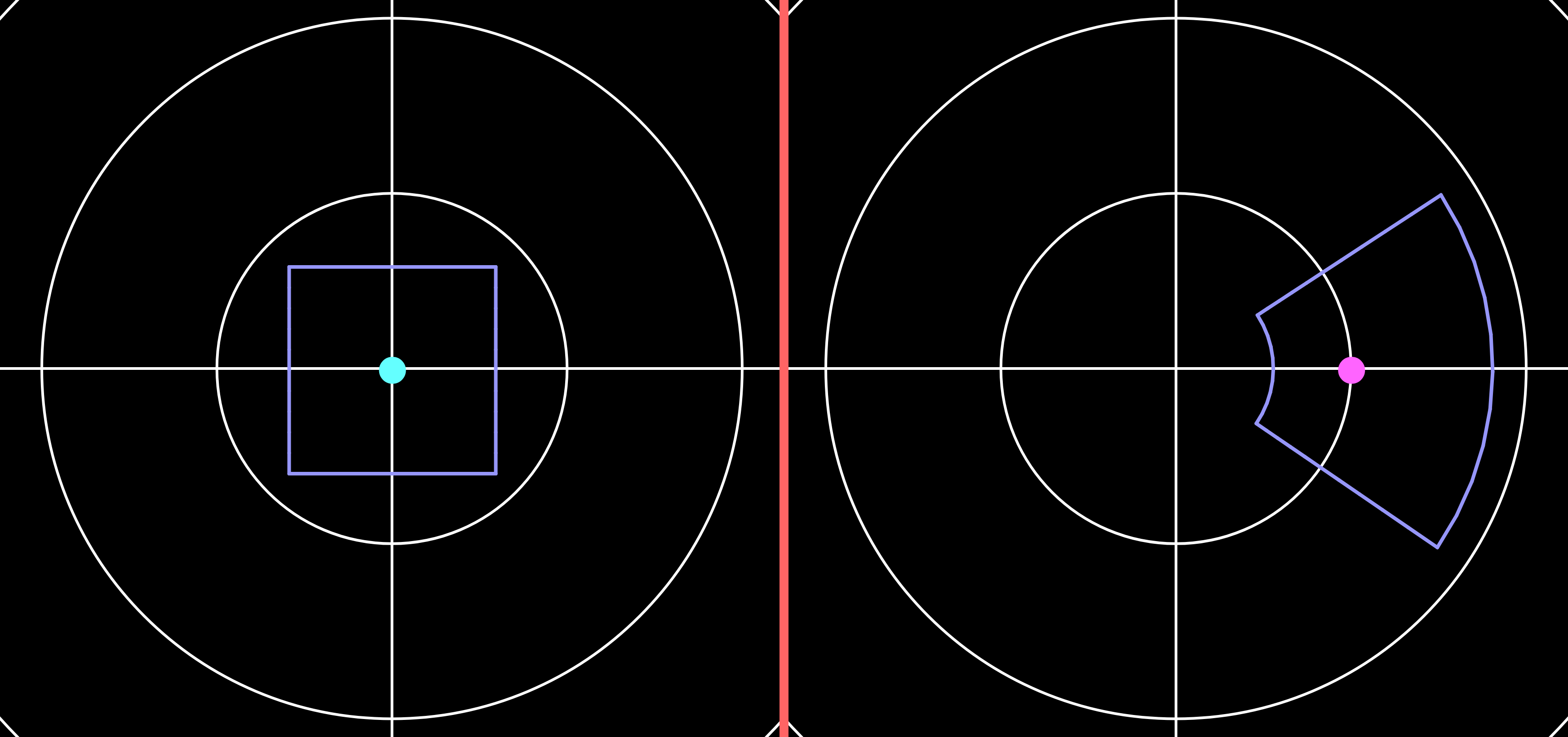
On the left we have the teal point at the origin, and a purple square around it. Since 
To view more such examples, with more elementary functions, go to:
https://openprocessing.org/sketch/1811203
In particular check out the simpler functions like 
Complex numbers as vectors:
The simplest visualization of a complex function 


- On the left: The identity function
. This means that the arrow at point
is, the bigger the arrow.
- On the middle: The function
is real, its square
is always positive, so that the arrow must point to the right. Similarly, when
is pure imaginary, its square is
is negative, so that the arrow points to the left.
- On the right: The function
. This function has two roots at
, which we can see as a pulling and pushing point in the image.
To check out more examples, go to:
https://openprocessing.org/sketch/1246491
Also, considering it as a flow field, you can view it dynamics here:
https://openprocessing.org/sketch/1244668
Complex numbers as colors:
Another interesting way to view complex number is by using their polar presentation 
More specifically, the color correspondence is according to following image:

- The radius
parameter controls the brightness. Near the origin the color is darker up to full black at the origin, and farther away it is more bright (more colorful).
- The argument
parameter controls the hue. As we rotate around the origin we see all the different colors, and in particular teal is for positive numbers, red is for negative, and similarly green\yellow for
with
and purple\blue for
.
For example, consider the functions 


- On the left:
as the black points. Between them the function is negative (e.g.
) so the color is red. On their right and left over the real line the parabola is positive, so it has teal color.
Note that when we go around each of the roots, we see all the color, and at the same order. - On the middle:
- On the right:
. Similar to the
example, but with two roots at
. Note that this function is positive on the real line, or in the color presentation it only has the teal color there.
To check out more examples, go to:
https://openprocessing.org/sketch/1246306
