Random walks and self similar sets

1. Introduction

In this post we consider an interesting mathematical process which can be easily simulated by a computer, and generates interesting pictures. A video version of this post can be seen in here (for now in Hebrew).

Let ${P_{0},P_{1}}$ and ${P_{2}}$ be the vertices of a triangle ${\Delta}$ and choose a random point ${q_{0}\in\Delta}$ in the triangle. Next, choose one of the triangle vertices uniformly at random and move ${q_{0}}$ half of the way towards it – we denote this point by ${q_{1}}$ . We now repeat this step infinitely many times – given the point ${q_{i}}$ we choose uniformly at random a vertex from $P_1,P_2,P_3$ , move $q_i$ half way towards that vertex and denote this point by $q_{i+1}$ .

The “limit” of this process produces a very interesting picture, as can be seen below.

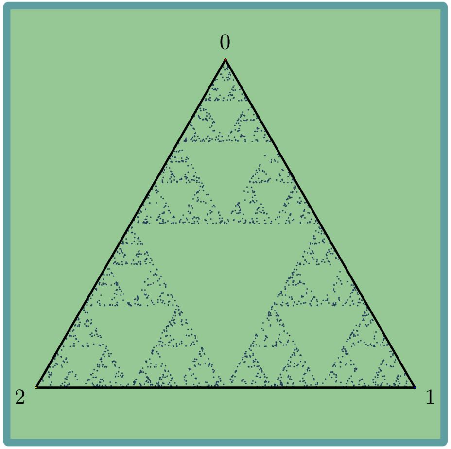
This process is called a random walk, since at each step we choose one of the vertices at random and continue according to this choice.

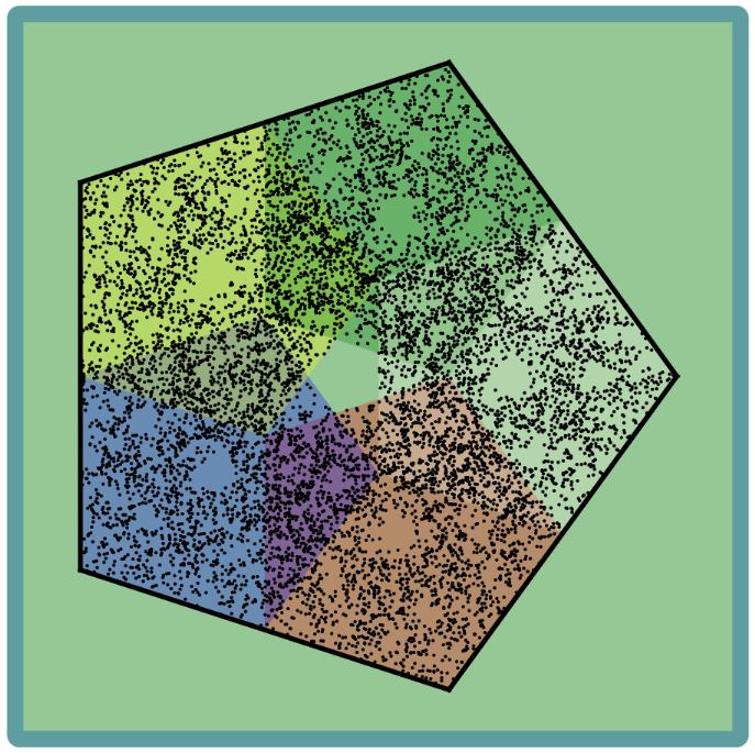
An interesting and natural question is if we can create more interesting pictures by starting with a different shape. For example, here are the result of the same process, but starting with a square and pentagon.

Random walk for square and pentagon with ratio 1/2.

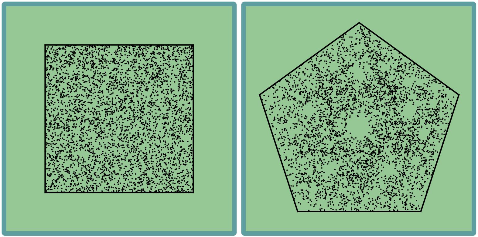
For the square, it seems like we just have a uniform distribution of points. For the pentagon the picture is not that simple – some places are empty (e.g. the center), while some are quite full.

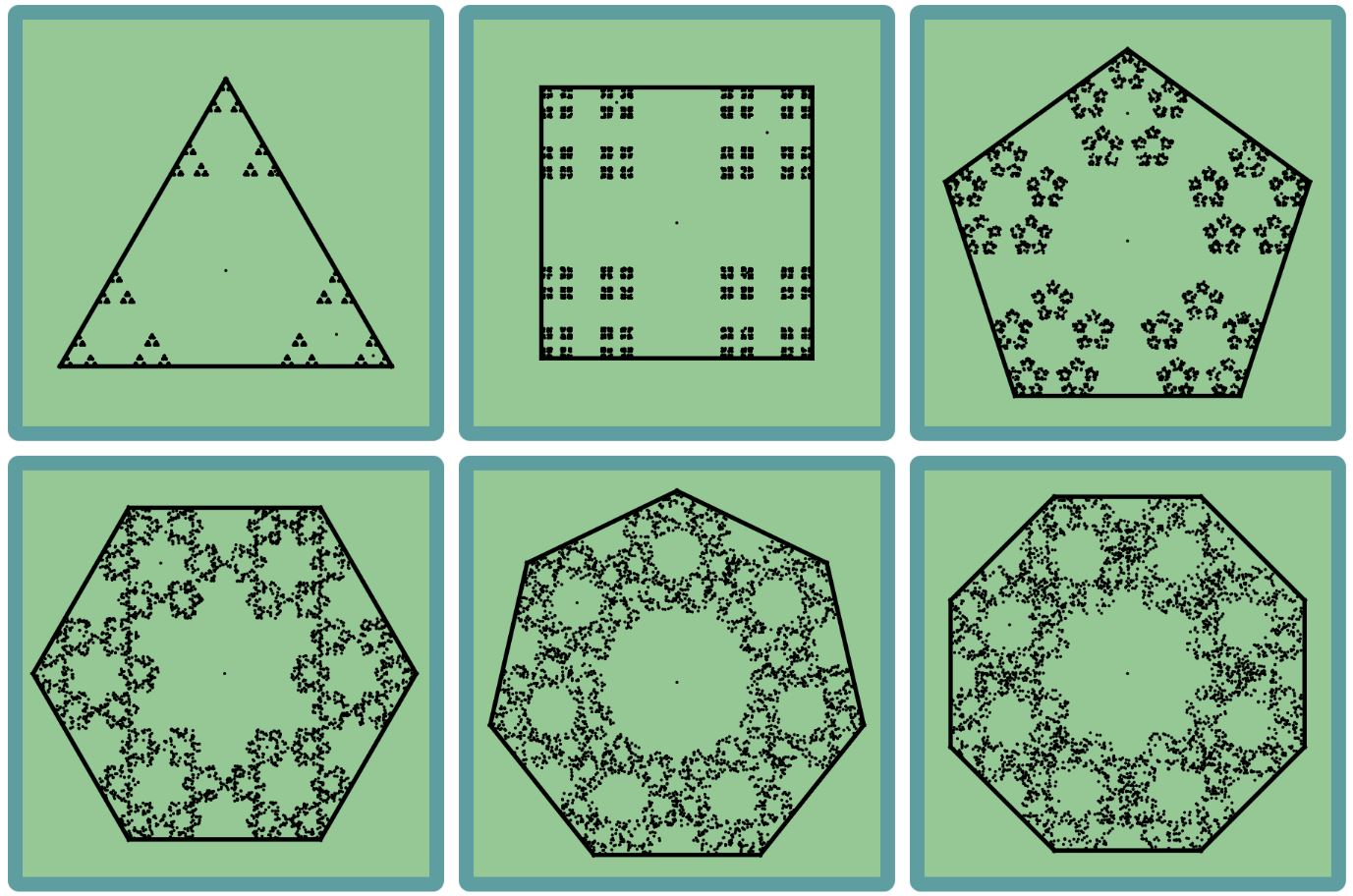
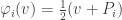
To better understand this process, instead of going half the way towards the vertices, we can use a different ratio. For example, if we move ${\frac{2}{3}}$ of the way, then we get the following images:

Random walk for ratio 2/3 for regular polygons

For ${3,4,5,}$ and ${6}$ vertices, we can clearly see small copies of the original polygon in the final image. The “type” of image is similar to what we have seen with the triangle and ratio ${\frac{1}{2}}$ . But for ${7}$ and $8$ it becomes more complicated and it is harder to recognize the smaller copies of the polygons.
On the other hand, we can rearrange the vertices a little different, still with ratio 2/3, and get an interesting picture like in the triangle.

Random walk for ratio 2/3 for the vertices in the blue circles

What we will try to do in this notes is to understand some of the mathematics behind these random walks and the final images that we get.

2. The Sierpinski Triangle

In this section we will concentrate on the process with ratio 1/2 when we start with the triangle. In this case the final image is called the Sierpinski triangle. In this section we will try to show that the only image possible (more or less) for this walk is the Sierpinski triangle

Before we start, recall that we have the following notation:

The points we get in this process are denoted by $q_0, q_1, q_2, ...$ .
Denote the three vertices of the triangle by $P_0, P_1$ and $P_2$ .
Denote the choices of the vertices by $w_i \in \{0,1,2\}$ for $i=1,2,3,...$ .

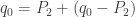
Note that moving towards a point $P$ with ratio $\lambda$ is exactly the function

$v \mapsto (1-\lambda)\cdot v + \lambda \cdot P$ .

In particular, in our case, the maps describing moving half the way towards the vertices are

$\varphi_i (v) = \frac{1}{2} (v+P_i)$ .

2.1. Simplifying the problem

As with many difficult problems in mathematics, and in general, the first step should be to try and simplify them as best as possible. Once we solve a simple version of the problem, we can hope to (1) get some intuition about the general solution and (2) use the simple result and extend it to get the full result.
In our case, instead of considering infinitely many steps simultaneously, let us consider just the first step, namely what can we say about ${q_{1}}$ ? While ${q_{0}}$ can be any point in the triangle, the point ${q_{1}}$ is more restricted and in particular it depends on the first vertex that we choose. More specifically, we can play around with the choice of ${q_{0}}$ , and see that ${q_{1}}$ must be in one of the small colored triangles as in the picture:

Can we show it directly from the process definition? Yes, but before we prove that let us consider a very special case – suppose that we chose ${P_{2}}$ in the first step and ${P_{1}=0}$ . In this case ${q_{1}=\frac{1}{2}\left(q_{0}+P_{2}\right)=\frac{1}{2}q_{0}}$ is just a contraction of ${q_{0}}$ – we divided in by ${2}$ . This is actually what happens in general, but instead of contracting towards ${0}$ we contract towards ${P_{0}}$ . To see this, write ${q_{0}=P_{2}+\left(q_{0}-P_{2}\right)}$ , namely start at ${P_{2}}$ and move by ${\left(q_{0}-P_{2}\right)}$ . Then

$\displaystyle q_{1}=\frac{1}{2}\left(q_{0}+P_{2}\right)=P_{2}+\frac{1}{2}\left(q_{0}-P_{2}\right),$

namely we start at ${P_{2}}$ and shrink the distance by a factor of 2.

This is of course true if we chose ${P_{0}}$ or ${P_{1}}$ in the first step. Namely, we have just shown that:

Corollary:

The function ${q_{0}\mapsto\frac{1}{2}\left(q_{0}+P_{i}\right)}$ is a contraction times ${2}$ towards ${P_{i}}$ .

Now the claim is clear. If we start with a triangle and shrink it by a factor of 2 towards one of its vertices, than we get a times 2 small triangle near the corresponding vertex.
We now know that the point ${q_{1}}$ is in one of the smaller triangles which we denote by ${\Delta_{0},\Delta_{1}}$ or ${\Delta_{2}}$ corresponding to the first vertex that we choose. What about the next point ${q_{2}}$ ? We can again try to see where it can fall, and do the same process as before, but let us keep our problem for now as simplified as possible and only ask in which colored triangle is it. Well, then we already did all the work above – the point ${q_{2}}$ will be in the colored triangle corresponding to our second vertex choice. Because we only consider this simple problem, namely which colored triangle contains the point ${q_{i}}$ , we can easily solve it – it is the triangle corresponding (only!) to the vertex choice in the ${i}$ -th step.

2.2. A partial result

Now that we have a very simple observation, let us study it and try to prove some partial result which will hopefully lead to the proof of our original result.
Under our simplified problem, we can only ask for each ${i}$ which colored triangle contains the point ${q_{i}}$ . After seeing ${N}$ points, a natural question to ask is how many points does each triangle contain, or more formally, for ${k=0,1,2}$ what is the size of the set

$\displaystyle \Omega_{k}^{N}=\left\{ 0\leq i\leq N\;\mid\;q_{i}\in\Delta_{k}\right\} .$

Running a simulation we can see that ${\left|\Omega_{k}\right|}$ is more or less ${\frac{N}{3}}$ for each ${k\in\left\{ 0,1,2\right\} }$ . Trying to quantify this “more or less” statement, we can increase ${N}$ and see that ${\left|\Omega_{k}^{N}\right|-\frac{N}{3}}$ doesn’t really stay this closed to zero. However, if we divide by ${N}$ , namely if we ask what is the ratio of the points in each triangle compared to the total number of points, we see that ${\frac{\left|\Omega_{k}^{N}\right|}{N}-\frac{1}{3}}$ do become closer and closer to zero as ${N}$ grows to infinity. Note that this result is very natural if we believe that the limit is going to be the Sierpinski triangle. Indeed, the Sierpinski triangle is a union of three copies of itself (almost disjoint) corresponding to our three contractions:

The Sierpinski triangle is a union of three small copies of itself

This claim about the orbit of our point is of course not always true. If for some reason we keep choosing only the bottom left vertex, then all of the point (except maybe the first which we ignore) will be in ${\Delta_{2}}$ (the yellow triangle). This means that ${\frac{\left|\Omega_{2}^{N}\right|}{N}=1}$ while ${\frac{\left|\Omega_{0}^{N}\right|}{N},\frac{\left|\Omega_{1}^{N}\right|}{N}=0}$ . But recall that in each step we choose a vertex uniformly at random, so the chances of such a choice is basically zero. Thus, the right formulation of what we mentioned above is that “with high probability ${\frac{\left|\Omega_{k}^{N}\right|}{N}\rightarrow\frac{1}{3}}$ for each ${k=0,1,2}$ ”.

Remark:

Notice the difference between what we know and what we claim. We know that in each step we choose uniformly at random, namely with probability ${\frac{1}{3}}$ each triangle. What we claim is that if we use this process of choices for long enough and then look back and count how many times we chose each triangle, then it is very likely to see close to ${\frac{1}{3}}$ of the choices for any triangle.

Let us give a proper formulation of this claim.
We begin by denoting the choice of indices for our vectors by ${w_{i}}$ . So for example, if we choose ${P_{1}}$ and then ${P_{2}}$ and then ${P_{1}}$ again, then ${w_{1}=1}$ , ${w_{2}=2}$ and ${w_{3}=1}$ . The claim that we proved above that the triangle containing ${q_{i}}$ only depends on the choice of vertex in the ${i}$ step can be written as follows:

Lemma:

For each ${i}$ we have that ${q_{i}\in\Delta_{w_{i}}}$ .

We can now write ${\Omega_{k}^{N}}$ as

$\displaystyle \Omega_{k}^{N}=\left\{ 1\leq i\leq N\;\mid\;w_{i}=k\right\} .$

This is a much better definition for ${\Omega_{k}^{N}}$ , because the ${w_{i}}$ are chosen independently while the ${q_{i}}$ depend on all the previous choices. Luckily for us, we showed that for the question of whether ${q_{i}\in\Delta_{k}}$ , we only need to know ${w_{i}}$ . Finally, we can write our claim about ${\left|\Omega_{k}^{N}\right|}$ as:

Claim:

For every ${\varepsilon>0}$ we have that

$\displaystyle \lim_{N\rightarrow\infty}P\left(\left|\frac{\left|\left\{ 1\leq i\leq N\;\mid\;w_{i}=k\right\} \right|}{N}-\frac{1}{3}\right|<\varepsilon\right)\rightarrow1.$

This claim should be understood as follows: there are many ways to choose our vertices in each step, but out side of a very small collection of bad choices, we are always spending ${\frac{1}{3}}$ of the time (with some ${\varepsilon}$ error) in each triangle. Moreover, as we take more and more steps the collection of bad choices becomes smaller and smaller compared to the total amount of choices (still for a fixed ${\varepsilon}$ ).
The experienced probabilists will immediately see that there is another way to formulate this limit which will follow from the well known (and elementary!) weak law of large numbers. The main trick here to think of ${\left|\left\{ 1\leq i\leq N\;\mid\;w_{i}=k\right\} \right|}$ as summing up 1’s for each time ${w_{i}=k}$ .
Let us fix ${k\in\left\{0,1,2\right\} }$ and define a random variable ${X_{i}}$ for each ${i}$ such that ${X_{i}=1}$ if ${w_{i}=k}$ and ${X_{i}=0}$ otherwise. In other words ${X_{i}}$ checks whether we are in the ${\Delta_{k}}$ trianagle or not after ${i}$ steps. Now, if we want to know how many times we have visited the ${k}$ -th triangle, then we only need to sum up those ${X_{i}}$ , namely

$\displaystyle \left|\left\{ 1\leq i\leq N\;\mid\;w_{i}=k\right\} \right|=\sum_{1}^{N}X_{i}.$

Thus, in the claim above we want to prove that

$\displaystyle \lim_{N\rightarrow\infty}P\left(\left|\frac{\sum_{1}^{N}X_{i}}{N}-\frac{1}{3}\right|<\varepsilon\right)=1.$

The term ${\frac{\sum_{1}^{N}X_{i}}{N}}$ is an average of random variables, and furthermore these are independent and identically distributed (i.i.d) random variables, with ${P\left(X_{i}=1\right)=\frac{1}{3}}$ (the chance of choosing the $k$ triangle) and ${P\left(X_{i}=0\right)=\frac{2}{3}}$ for each ${i}$ . The “average” of a single such ${X_{i}}$ , namely the expectation is

$\displaystyle \mathbb{E}\left(X_{i}\right)=1\cdot P\left(X_{i}=1\right)+0\cdot P\left(X_{i}=0\right)=\frac{1}{3}.$

The weak law of large numbers say that if the ${X_{i}}$ are ${i.i.d}$ and the “average” of a single ${X_{i}}$ is ${c}$ , then with high probability the average of all the ${X_{i}}$ together is close to ${c}$ .

Theorem (Weak Law of Large Numbers):

Let ${X_{i}}$ be i.i.d with expectation ${\mu}$ , then for any ${\varepsilon>0}$ we have that

$\displaystyle \lim_{N\rightarrow\infty}P\left(\left|\frac{\sum_{1}^{n}X_{i}}{N}-\mu\right|<\varepsilon\right)=1.$

2.3. Improving the partial result

What we did so far is:

We tried to simplify our problem by ignoring the “infinitely many points” and only consider the first two point.
This led us to consider the 3 small contractions of the original triangle.
Restricting our attention only to these triangles, we conjectured that the orbit of the point spend around ${\frac{1}{3}}$ of its time in each triangle.
We got a little bit into the details of this claim and added the “with high probability” part.
Finally, we showed that our simplified conjecture follows from the Weak Law of Large Numbers.

Now we can try to repeat this proof process but with a little bit more information. Considering the first 3 points, we can show that the third point must be in one of nine very small triangles, depending on the first 2 choices of vertices:

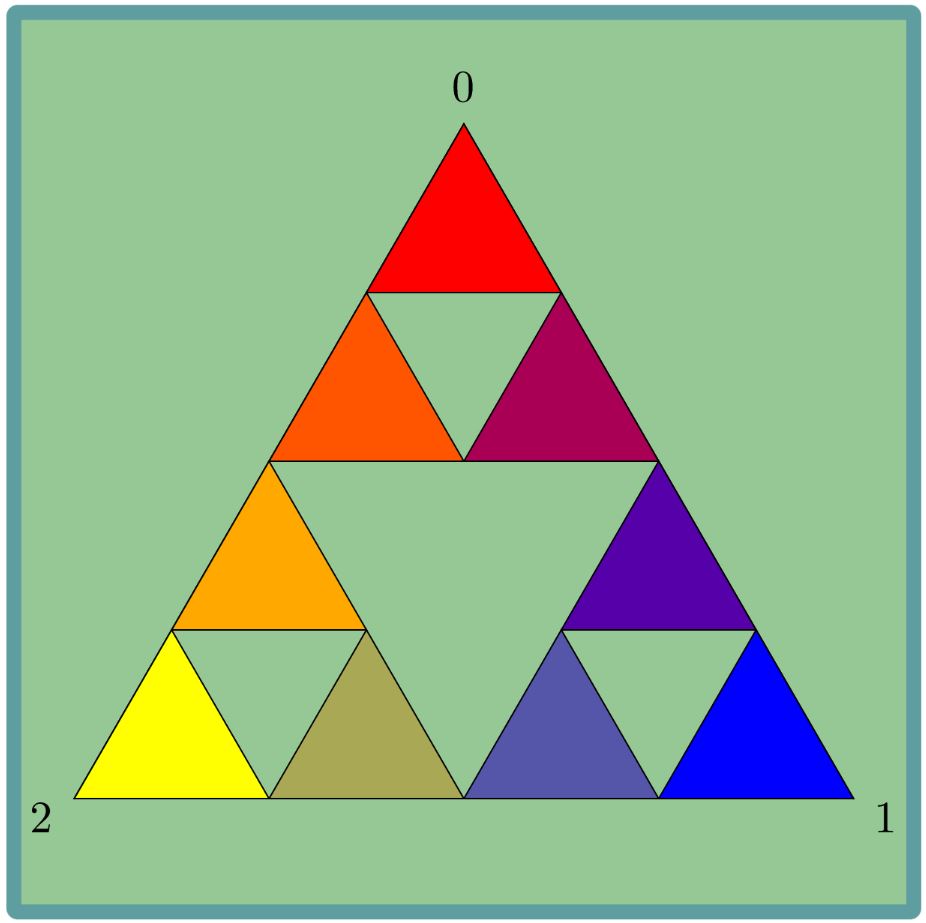
As before, we can again ask how many times we visit each triangle, and a simulation will show that we spend around ${\frac{1}{9}}$ of the time in each triangle. In the previous step we had the triangles ${\Delta_{0},\Delta_{1},\Delta_{2}}$ , and ${q_{i}}$ was in ${\Delta_{k}}$ if and only if ${w_{i}=k}$ . Generalizing this notation, we can denote the smaller triangles in the picture about by ${\Delta_{k_{1},k_{2}}}$ such that ${q_{i}\in\Delta_{k_{1},k_{2}}}$ if the two vertex choices before we get to ${q_{i}}$ are ${w_{i}=k_{2}}$ and ${w_{i-1}=k_{1}}$ . Equivalently, we have the following generalization of out previous lemma.

Lemma:

For all ${i\geq2}$ we have that ${q_{i}\in\Delta_{w_{i-1},w_{i}}}$ .

Continuing to follow the previous step, let us fix ${k_{1},k_{2}\in\left\{ 0,1,2\right\} }$ and define random variables ${Y_{i}}$ such that ${Y_{i}=1}$ if ${q_{i}\in\Delta_{k_{1},k_{2}}}$ and ${Y_{i}=0}$ otherwise. Thus, counting how many of the ${q_{i}}$ for ${2\leq i\leq N}$ are in ${\Delta_{k_{1},k_{2}}}$ we get the expression ${\sum_{2}^{N}Y_{i}}$ . So saying that we spend around ${\frac{1}{9}}$ of the time in each triangle can be formulated as

$\displaystyle \forall\varepsilon>0\qquad\lim_{N\rightarrow\infty}P\left(\left|\frac{\sum_{2}^{N}Y_{i}}{N-1}-\frac{1}{9}\right|<\varepsilon\right)=1,$

where as before

$\displaystyle \mathbb{E}Y_{i}=1\cdot P\left(Y_{i}=1\right)+0\cdot P\left(Y_{i}=0\right)=\frac{1}{9}.$

Unfortunately, we cannot use directly the Weak Law of Large Numbers, since the ${Y_{i}}$ are dependent. Indeed, because ${Y_{i}}$ correspond to the ${i-1}$ and ${i}$ choices and ${Y_{i+1}}$ correspond to the ${i}$ and ${i+1}$ choices. Fortunately if ${j>i+1}$ then ${Y_{i}}$ and ${Y_{j}}$ are independent, so we can hope for a generalization of the weak law.
Recall that we can “measure” how much two random variables are dependent by computing their covariance

$\displaystyle Cov\left(X,Y\right)=\mathbb{E}\left(XY\right)-\mathbb{E}\left(Y\right)\mathbb{E}\left(X\right),$

and in particular ${Cov\left(X,Y\right)=0}$ is equivalent to ${X,Y}$ being independent.
In our case ${Cov\left(Y_{i},Y_{j}\right)=0}$ if ${\left|i-j\right|>1}$ , and whatever $Cov(Y_i,Y_{i+1})$ is, it is easily seen to be independent of $i$ .

In order to generalize the Weak Law of Large Numbers, let us first recall its proof using Chebyshev’s inequality.

Theorem (Chebyshev’s inequality):

Let $X$ be a random variable with finite expectation $\mu$ and variance $\sigma$ . Then for any $\varepsilon>0$ we have that:

$P(|X-\mu|>\varepsilon)\leq \frac{\sigma^2}{\varepsilon^2}$

This already looks similar to the weak law. Just put $X_N=\frac{\sum_1^N Y_i}{N}$ where the $Y_i\sim Y$ are identically distributed with expectation $\mu$ , to get that $\mathbb{E}(X_N)=\mu$ also so that

$P(|\frac{\sum_1^N Y_i}{N}-\mu|>\varepsilon)\leq \frac{\sigma(X_N)^2}{\varepsilon^2}$

If we can only show that $\sigma(X_N)^2$ goes to zero as $N\to \infty$ , then we are done. This follows from the fact that

$\sigma(X_N)^2 = \frac{1}{N^2} (\sum_{i,j=1}^{N}Cov(Y_i,Y_j))=\frac{1}{N^2}(N\sigma(Y)^2+2\sum_{1\leq i<j\leq N}Cov(Y_i,Y_j))$

In the case where the $Y_i$ are independent, all of the $Cov(Y_i,Y_j),\;i\neq j$ are zero, so that $\sigma(X_N)^2=\frac{1}{N}\sigma(Y)^2\to 0$ . But even in general, if we can show that the sum $\sum _{i<j} Cov(Y_i,Y_j)$ is not to big, then the limit is still zero. I will leave the rest of the proof to the reader, to show that the Weak Law of Large numbers still holds for our two steps process, and actually this can now be straight forward generalized to any $T$ steps.

To conclude, we can keep subdivide our triangles, each one to 4 smaller triangles, and remove the middle one, and for each such configuration the orbits of our point will spend (up to some $\varepsilon>0$ -error) the same amount of time in each triangle.

So now we know that if we fix a triangle size, the orbit spends the same amount of time in each triangle. The only shape that has this property is the Sierpinski triangle, so whatever the definition of “limits of random walks” is, the limit here should be the Sierpinski triangle.

2. The other examples

We saw that the random walk process implied that “its limit” should be “equality distributed” in our first three colored triangles, and then after the second step in the nine smaller triangles, then $3^3$ triangles, $3^4$ triangles etc. Since the Sierpinski triangle satisfy this – it is a disjoint union of its three (respectively 9,27,…) smaller contractions – it must be the “limit”. We shall give a proper definition for the limit in a future post, but for now, let’s see if we can use our intuition to understand the rest of the example.

The square is a disjoint union of four smaller (by a factor of 2) squares near its vertices. Thus, just like the Sierpinski triangle, it must be the limit of our random process with 4 vertices.

Square is as a disjoint union of 4 small squares

On the other hand, for the pentagon, the 5 contractions are not disjoint, so we do not expect a “simple” picture as in the case of the triangle and square. Note how there seem to be more points where the smaller pentagons overlap.

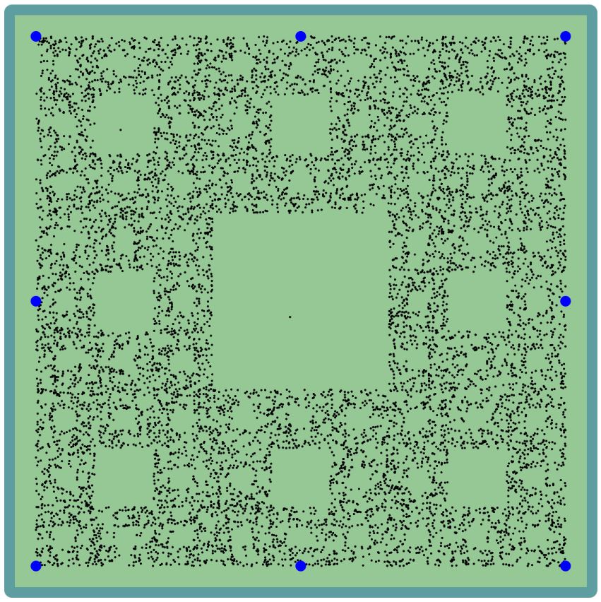
When we switched to ratio $\frac{2}{3}$ , the contractions are smaller (by a factor of $1-\frac{2}{3}=\frac{1}{3}$ ), so it is easier for them to be disjoint. This is why we can nice and “simple” picture for up to 6 vertices.

Six contraction by a factor of $\frac{1}{3}$ of the hexagon

Finally, when we rearranged the 8 vertices in a square shape, it corresponded to 8 disjoint contractions of a square, thus giving us a final image with smaller and smaller squares, very similar to what we got in the Sierpinski triangle.

All the images that we saw so far are call “self similar sets”, since they are similar to themselves after the corresponding contractions. You can now try running your own simulations with random walk and see what images you can come up with. In particular, when you start with a “nice” shape and where the contractions produce disjoint sets, the final image usually seem more interesting. In general these processes usually use more general map and not just contractions, and in particular they use translations and rotations. In a future post, where we will ask what is exactly the limit of a random process, we will discuss this more general setting.