Random walks on graphs

Imagine going to a new amusement park for the first time. Once you get there, you go to the first ride that you see, and when you finish it, you randomly choose one of the roads leaving it and follow it until you reach another ride. You continue like this for a long time – every time you go on a ride, then choose a random road (might even go back on the same road that you came) and walk on it until you reach your next ride.

After doing this for a long enough time, on which ride would you go on the most? Go on the least? And how are these questions connected to eigenvectors and eigenvalues?

People randomly enjoying themselves in an amusement park.

Go to https://www.openprocessing.org/sketch/829178 to see and interact with the animation above.

Two (nontrivial) examples:

In order to get some intuition about this problem, let’s consider some simple examples.

The simplest case is when there is only one ride, but then there is really nothing to prove. After that, we might have two rides connected by a road. In this case you will just alternate between the two rides, and you will get stuck like this for the rest of eternity.

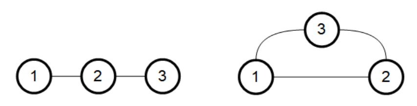
We now go to the first nontrivial case – there are 3 rides in the park. We may assume that all the rides in the park are connected by roads, since otherwise there will be rides that we can never reach, and this is just cruelty. So under this assumption we have two options – either each two rides are directly connected by a road, or we have one ride which is connected to the other two, which are not directly connected.

A not amusing presentation of two amusement parks

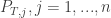
Suppose first that we are in the $1-2-3$ case on the left, where there is no direct road from 1 to 3. It is then easy to see that in our journey through the park, we alternate between being on ride 2 and being on one of the rides in $\{1,3\}$ . This means that if we went on $m$ rides, then at $m/2$ of the times we were on ride 2. After each time we go on this ride, we go to either ride 1 or ride 3 with equal probability, so we expect to visit each of these rides around $\frac{1}{2} \frac{m}{2}=\frac{m}{4}$ times.

In the cycle case on the right, we no longer have this alternation trick like before, but we can still try to adapt the second argument. Suppose that we went $n$ times on the three rides, and we set $m_1, m_2$ and $m_3$ to be the number of times we went on rides $1, 2$ and $3$ respectively. If we are on ride 1, then with probability $\frac{1}{2}$ we will next go to ride 2, and otherwise (also with probability $\frac{1}{2}$ ) we will go to ride 3. We can similarly do these arguments for the other rides.

Looking at it from the other way around, if we are now on ride 1, then with equal probabilities ( $=\frac{1}{2}$ ) we came from either ride 2 or ride 3. Thus if we know what are $m_2$ and $m_3$ , then we expect $m_1$ to be more or less $\frac{1}{2}m_2+\frac{1}{2}m_3$ (assuming, the number of times we visit each ride doesn’t change to much after one such step). The same argument can be said for $m_2$ and $m_3$ so we expect the tuple $(m_1,m_2,m_3)$ to “almost” satisfy the equation:

$\left( \begin{array} {ccc} m_1 \\ m_2\\ m_3\end{array} \right) = \left( \begin{array} {ccc} 0 & 1/2 & 1/2 \\ 1/2 & 0 & 1/2 \\ 1/2&1/2&0 \end{array} \right) \cdot \left( \begin{array} {ccc} m_1 \\ m_2\\ m_3\end{array} \right)$

But this equation is none other than asking to find an eigenvector for the matrix above, corresponding to the eigenvalue 1. For this matrix, it is not hard to check that the eigenspace for 1 is spanned by the constant vector $(1,1,1)^{tr}$ . This means, that in our original question, we will visit each ride around the same number of times (because $(m_1,m_2,m_3) \sim k(1,1,1) )$ .

This is a good place for a sanity check. In the first graph we had two leaves and one node with two edges, and in a sense we saw this structure in our solution ( $\frac{n}{4}$ visits for the leaves and $\frac{n}{2}$ in the middle node). The second graph was completely symmetric, so in the solution we saw that each node is visited the same amount of time.

The mathematical model:

Now that we have a little bit of intuition, let’s try to build a mathematical model for a general amusement park.

We begin by thinking about the park as a graph, where the vertices are the rides numbered by $1,2,...,n$ , and the edges are the connecting roads. We will write $i\sim j$ if there is an edge from vertex $i$ to vertex $j$ . As we mentioned before, we may assume that our graph is connected – any two rides are connected (not necessarily directly) via a sequence of roads. Given the $i$ -th vertex, we denote by $d_i$ its degree (=number of edges which touch it). This means that when we leave the vertex $i$ , we choose one of its edges uniformly to lead us to the next ride, namely, the probability to choose each of these edges is $\frac{1}{d_i}$ . To visualize this random choice we make our graph into a directed graph, and on each outgoing edge we write the probability of choosing that edge when leaving the vertex:

This image has an empty alt attribute; its file name is 4graph.png — The probability of choosing an edge leaving vertex $i$ is $1/d_i$ .

The probability of choosing an edge leaving vertex $i$ is $1/d_i$ .

Since our system is probabilistic – we keep choosing roads at random – and as such we can only ask probabilistic questions (e.g. which ride\vertex do we expect to visit the most). There are now several ways to think about how the dynamics of our system works.

One way, is instead of having just one person travelling on the graph, we have $N$ people doing it where $N$ is very large and then follow the quantities of people in each vertex over time, which we measure by $T=0,1,2,3,...$ . For example, in the graph above vertex 1 is connected to vertices 2 and 3 so that, so if there are $m$ people there at time $T$ , then at time $T+1$ about $\frac{m}{2}$ will move to each of the vertices 2 and 3.

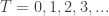
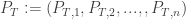
The second way to view this system, is as above, but instead of counting people in each vertex, we measure their part out of the whole visitors in the park (so we will have $\frac{m}{N}$ instead of just $m$ in the previous example). If we denote by $P_{T,i}$ how much of all of the people are in vertex $i$ at time $T$ , then we will get that $\sum_{i=1}^n P_{T,i} = 1$ at each time $T$ . In other words, the vector $P_T:=(P_{T,1}, P_{T,2}, ..., , P_{T,n})$ is a probability vector. With this new notation, we can also think about the term $P_{T,i}$ as the probability of being in vertex $i$ at time $T$ . Finally, at time $T=0$ we start in a single vertex, so up to reordering, we may assume that $P_0 = (1,0,0,...,0)$ .

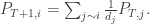
Now that we have a presentation of our states at each point in time, we want to find the relation between consecutive times. In order to compute $P_{T+1,i}$ we need to know first all the $P_{T,j}, j=1,...,n$ at time $T$ and then ask what is the probability of moving from vertex $j$ to vertex $i$ . Since we choose edges (=roads) at random, in order for this probability to be nonzero, first we must have an edge connecting these two vertices. Second, our choice of edge leaving vertex $j$ is uniform, so we will choose the one leading to vertex $i$ with probability $\frac{1}{d_j}$ , where $d_j$ is the degree of vertex $j$ . Then we collect all the probabilities together to get

$P_{T+1,i} = \sum_{j \sim i} \frac{1}{d_j} P_{T,j}.$

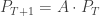
The equation above tells us that the vector $P_{T+1}$ can be computed from $P_T$ in a linear way. More precisely, if we define the matrix $A\in M_n(\mathbb{R})$ to be such that

$A_{i,j}=\begin{cases}\frac{1}{d_{j}} & i\sim j\\0 & else\end{cases},$

then we will get that $P_{T+1} = A\cdot P_T$ .

For example, let us return to our two graphs with 3 vertices. In the case of the path $1-2-3$ , the degrees are $d_1=1, d_2=2$ and $d_3=1$ and the matrix will be

$\left( \begin{array} {ccc} 0 & 1/2 & 0 \\ 1 & 0 & 1 \\ 0&1/2&0 \end{array} \right).$

So if, for example, we are at the first ride, namely we start at $e_1 = (1,0,0)^{tr}$ , then next we will be on the second ride $Ae_1=e_2 = (0,1,0)^{tr}$ . After finishing with this second ride we have that $A^2e_1=Ae_2= (1/2,0,/12)^{tr}$ so with probability $1/2$ we will be in either the first ride or the third. Equivalently, we can think of that as having half of the people in the park on ride 1 and half on ride 3.

In the case of the circle, each vertex is connected to the other two vertices, and the matrix will be the one then we saw before:

$\left( \begin{array} {ccc} 0 & 1/2 & 1/2 \\ 1/2 & 0 & 1/2 \\ 1/2&1/2&0 \end{array} \right).$

Eigenvectors and eigenvalues

Now, that we have our mathematical modeling with the equation $P_{T+1} = A\cdot P_T$ , we can use induction to conclude that $P_T = A^T \cdot P_0$ . In our original question we asked which ride we visited the most, which with our new notation becomes for which $i$ the value $P_{T,i}$ is maximal? Of course, this index depends on $T$ . Moreover, as we have seen with the 1-2-3 graph before, this index can alternate depending on whether $T$ is even or odd. Actually computing $P_T$ or $A^T$ can be rather hard in general, but luckily for us, linear algebra has exactly the tool to try and solve this problem – eigenvectors and eigenvalues.

Recall that an eigenvector $v\neq 0$ corresponding to an eigenvalue $\lambda$ for the matrix $A$ is a vector satisfying $Av = \lambda v$ . For such vector, it is very easy to compute $A^T v$ which is simply $\lambda^T v$ . More generally, if $v = \sum a_i v_i$ where $v_i$ are eigenvectors corresponding to eigenvalues $\lambda _i$ , then $A^T v = \sum a_i \lambda _i^T v_i$ . Finally, we say that $A$ is diagonalizable if it has some basis of eigenvectors, in which case we can use the argument above for every vector. In particular, we could use this to find what is $P_T = A^T P_0$ .

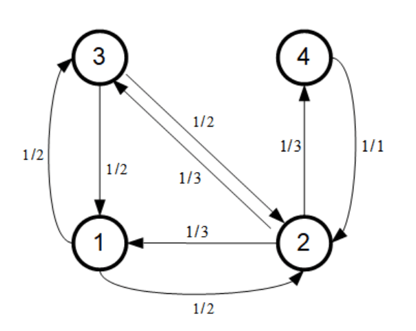
Finding the eigenvalues is usually done by finding the roots of the characteristic polynomial, which is not an easy task in general. However, our matrix is not any general matrix – it comes from a graph. To visualize what is an eigenvector $(v_1,...,v_n)$ we attach each $v_i$ to the corresponding $i$ -th vertex, and then $Av=\lambda v$ simply says that for each $i$ we have that $\lambda v_i$ is the “average” of the $v_j$ entering it from neighboring vertices. However, this is not the standard average – the weight that we attach to each $v_j$ is the weight that we have on the corresponding edge it moves on.

For example in the graph above, $\lambda v_1$ should be equal to $\frac{1}{3} v_2 + \frac{1}{2} v_3$ (blue arrows), while $\lambda v_2 = \frac{1}{2} v_1 + \frac{1}{2} v_3 + \frac{1}{1} v_4$ (red arrows).

In order to really be an average, the sum of the weights should be one, which is not the case. However, if instead of looking on edges entering the vertex, we look on edges leaving the vertex, we would instead get that $\lambda u_1 = \frac{u_2 + u_3}{2}$ and similarly $\lambda u_2 = \frac{u_1 + u_3 + u_4}{3}$ , which is the uniform average over the neighbors. In our matrix notation, inverting the direction of the edges is the same as transposing the matrix (check it!), and what is nice about taking the transpose, is that $A$ and $A^{tr}$ have the same eigenvalues (this is because transposing a matrix doesn’t change the determinant). Thus, just to find the eigenvalues, we can consider this problem instead – look for a vector $(u_1,...,u_n)$ and $\lambda$ such that for each $i$ , we have that $\lambda u_i$ is the uniform average of the $u_j$ with $i\sim j$ .

Stochastic matrices:

Taking the constant vector $\bar{1} = (1,...,1)$ , we immediately see that it corresponds to the eigenvalue 1. Indeed, the number 1 is always the average of 1’s! In matrix notation we get that $\bar{1} \cdot A = \bar{1}$ . Matrices which satisfy this condition are called (left) stochastic matrices. This condition already tells us that 1 is an eigenvalue (from the right) of our matrix also. The eigenvectors of $A$ and $A^{tr}$ are usually different, though once we have the eigenvalue 1, finding an eigenvector is a simple problem of solving linear equations, e.g. $Av=v$ , which we all know and love, so this will not be a problem.

What about other eigenvalues? Using our new point of view which uses uniform averages, we can apply a new method – if a number $a$ is an average of $a_1,...,a_k$ , then it cannot be strictly larger (resp. smaller) than all of these $a_i$ . More specifically, suppose that $\bar{u}=(u_1,...,u_n)$ is an eigenvector for an eigenvalue $\lambda$ and suppose that $|u_k|\neq 0$ is the maximum in absolute value. Then we will get that

$|\lambda| |u_k| = \frac {|\sum_{j\sim k} u_j|}{d_k} \leq \frac {\sum_{j\sim k}|u_j|}{d_k}\leq |u_k|,$

and in particular we conclude that $|\lambda|\leq 1$ . Thus, not only 1 is an eigenvalue, all the rest of the eigenvalues are smaller in absolute value. Let us show a little bit stronger result.

Suppose that we find some eigenvector with $|\lambda|=1$ . This means that both of the inequalities above must be equalities. From the equality in the triangle inequality we get that the $u_j$ with $j\sim k$ must have the same sign, and from the second inequality they must also satisfy $|u_j|=|u_k|$ . In particular this means that the neighbors of the $k$ -th vertex also have maximal absolute value for $|u_j|$ , so we can apply the same argument for them and their neighbors. Repeating this process as many times as we need, and using the fact that our graph is connected, we conclude that all the $|u_j|$ are the same.

Of course, if the vector $(u_1,...,u_n)$ is constant, then its entries in absolute values are also constant, but is this the only solution? The answer for this is false, and indeed the vector $(1,-1,-1,1)$ is an eigenvector of the eigenvalue -1 for the following graph:

The red $\pm 1$ are the entries from the eigenvector

The red $\pm 1$ are the entries from the eigenvector

The graph above is bipartite – we can separate the vertices to two sides $V=V_0 \sqcup V_1$ (according to the sign of $u_i$ , namely $\{1,4\}$ and $\{2,3\}$ ) and there are no edges between two vertices which are either both in $V_0$ or both in $V_1$ . This means that when we travel the graph, we alternate between the two sides of the graph (just like in the $1-2-3$ graph from before). I will leave it as an exercise to show that a similar result holds in general – the matrix $A$ has eigenvalue -1 if and only if its graph is bipartite, and then the signs of the entries of the eigenvector correspond to the two sets in the decomposition of the vertices.

For clarity of this exposition, we will ignore these bipartite graphs, which means that our graph has some cycle of odd length. Note that this will always be the case, if we also let the people stay on the same ride, because then we will have self loops which have length 1. Anyway, if the graph is not bipartite, then we have just seen that 1 is an eigenvalue, and the rest of the eigenvalues are strictly smaller in absolute values. Moreover, the eigenvectors of the eigenvalue 1 are just the constant vectors. In the linear algebra notation, this means that the geometric multiplicity of the eigenvalue 1 is 1.

Up until now we used the fact that the sum of the weights leaving each vertex sum up to 1 (though we didn’t really need them to be equal!). If you paid enough attention, you also saw that in our triangle inequality argument we also used the fact that these weights are nonnegative. Matrices with nonnegative entries play crucial roles in many problems, and the result above can be generalized to such matrices. This result is known as the Perron Frobenius theorem. In our case, among other things, this theorem shows that not only the geometric multiplicity of 1 is 1, but also its algebraic multiplicity is 1, or in other words 1 is a simple root of the characteristic polynomial of $A$ .

As mentioned before, the eigenvalues of $A$ and $A^{tr}$ are the same, so $A$ also has 1 as its eigenvalue and the rest of its eigenvalues have strictly smaller absolute values. Actually, one can show that transposing the matrix doesn’t change the multiplicities, both algebraic and geometric, of the eigenvalues, so 1 is a simple eigenvalue of $A$ also.

Back to dynamics:

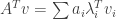
Let us denote by $v_1$ the unique eigenvector (up to a scalar multiplication) of $A$ corresponding to $\lambda_1=1$ . Assume that $A$ is actually diagonalizable, and let $v_2,...,v_n$ be eigenvectors for the eigenvalues $\lambda_2,...,\lambda_n$ such that $\{v_1,...,v_n\}$ is a basis for $\mathbb{R}^n$ . If $v\in \mathbb{R}^n$ is any vector, then we can write it as $v = \sum_1^n \alpha_i v_i$ . We then get that

$A^T v = \sum_1^n \alpha_i A^T v_i = \sum_1^n \alpha_i \lambda_i^T v_i = \alpha_1 v_1 + \sum_2^n \alpha_i \lambda_i^T v_i.$

Using the fact that $|\lambda_i|<1$ we get that $\lambda_i^T \to 0$ as $T\to \infty$ . Thus, for all $T$ big enough we have that $A^T v$ is $\alpha_1 v_1$ up to a small error which goes to zero as $T\to \infty$ . In other words, up to this small error we know what is $A^T v$ for all big enough $T$ , which is exactly what we wanted to know. Moreover, we didn’t even needed to find the rest of the eigenvalues and their eigenvectors! Well, almost. We still need to find what is $\alpha_1$ . Fortunately, there is a nice trick when dealing with eigenvectors of a matrix $A$ if we know the eigenvectors of it transpose.

Lemma: If $u,v\in \mathbb{R}^n$ satisfy $Av=\lambda v$ , $A^{tr}u=\mu u$ with $\lambda \neq \mu$ , then $u^{tr}\cdot v = 0$ .

Proof: Consider the scalar $u^{tr}Av$ . Using our assumption we get that

$\mu u^{tr}\cdot v = (A^{tr}u)^{tr}v = u^{tr}Av = \lambda u^{tr}\cdot v.$

Since $\lambda\neq \mu$ we conclude that we must have that $u^{tr}\cdot v=0$ . $\square$

Returning to our matrix $A$ coming from the graph, we already computed $v_1$ which is the eigenvector for 1, and we assumed that there are eigenvectors $v_2,...,v_n$ corresponding to eigenvalues which are not 1. On the other hand, we know that $\bar{1}=(1,...,1)$ satisfies $\bar{1} \cdot A =\bar{1}$ (so it is an eigenvector for $A^{tr}$ ). It follows that $\bar{1}\cdot v_i =0$ for all $i>1$ . Thus, if $v = \sum_1^n \alpha_i v_i$ , then

$\bar{1}\cdot v = \sum_1^n \alpha_i \bar{1}\cdot v_i = \alpha_1 \bar{1}\cdot v_1.$

If we know that $\bar{1}\cdot v\neq 0$ , then both of $\alpha_1$ and $\bar{1}\cdot v_1$ are nonzero, and we get that $\alpha_1 = \frac{\bar{1}\cdot v}{\bar{1}\cdot v_1}$ . Recall that in our original problem, the vector $v=P_0$ is $(1,0,...,0)^{tr}$ , so that $\bar{1}\cdot {v} = 1$ .

To summarize, we get that

Theorem: As $T\to \infty$ we get that

$A^T v \to \frac{\bar{1}\cdot v}{\bar{1}\cdot v_1} v_1$ .

Note that while the proof for the theorem above was not trivial, in order to apply it, we only need to know what is $v_1$ , and in order to find it we only need to know how to solve a simple system of linear equations $Av_1 = v_1$ , or equivalently $(A-I)v_1 = 0$ .

The last result followed from the fact that our matrix was stochastic, and can be interpreted in a probabilistic language. Indeed, we defined our process so that each of the $P_T$ will be probability vectors (their entries are nonnegative and sum up to 1) so the same is true for the limit. Hence, we just need to choose $\alpha_1$ to normalize $v_1$ so its entries will sum up to 1 (or more generally, sum up to the same sum of the entries of $v$ ). The algebraic reason for this follows from the fact that $\bar{1} A = \bar{1}$ and $A$ has nonnegative entries. Indeed, if $v$ is a probability vector, then the entries of $Av$ are nonnegative and $\bar{1}(Av)= (\bar{1} A)v=\bar{1} v = 1$ , so that $Av$ is also a probability vector.

This almost completes the proof, however we did assume along the way that $A$ is diagonalizable. The result above still holds if this is not true, but for that we need some more tools, e.g. the Jordan form of a matrix, and I will leave it for another time. I will just mention that if our graph is $d$ -regular, namely all the degrees in the graph are the same and equal to $d$ , then the matrix $A$ is symmetric. In this case it is true that it is diagonalizable, and moreover it has a base of eigenvectors which form an orthonormal base. This result is usually known as the Spectral Theorem.

Some more applications and conclusion

The problem of the amusement park is quite similar to many other “real life” problems. For example we can consider people surfing the web by going from site to site by clicking links “randomly” in each site. Here too we can ask which site do we expect them to visit the most, thus in a way “defining” what is a popular website.

Similarly, we can think of a system of players (=vertices), such that on each turn they pay a certain percentage of their money to other players (=weights on the edges). The same model will help here as well, though we will probably want to add self loops, so players can keep some of their money each turn. We can then ask which player will have most of the money after long enough time.

There are many more such problems, and I encourage you to find some by yourself. Mathematically speaking, we combined the fields of linear algebra, combinatorics and probability to get some interesting results. The next step after this is to work with more “symmetric” systems where the random choices have some structure by themselves. Probably one of the most famous problem is mixing a deck of card, where at each time you choose one of a small set of types of deck mixing (e.g. switch the first and second card, put the top card at the bottom of the deck , etc.). This type of problems usually add to the mix the field of abstract algebra and in particular groups and their representations, and at least for me, this combination is one of the most beautiful parts of mathematics.