Radars and the Chinese Remainder Theorem

The radar is a detection system that was developed before and during World War II for military uses, though by today it has many other applications including, for example, astronomical and geological research. The name radar is an acronym for RAdio Detection And Ranging, and as its name says, it uses radio waves to detect targets. In this post we will try to understand one of the basic ideas behind the operation of the radar, which while it seems quite simple at first glance, when we start to try to understand the details, we encounter an interesting problem. In order to solve it we will need to use a mathematical theorem first formulated by the Chinese mathematician Sunzi from the 3rd century AD.

For an English video version of this post – https://youtu.be/OoWoxBhixDI

For a Hebrew video version of this post – https://youtu.be/30CEOB_j3Ag

Let us begin with this basic idea. Suppose that we are in the control center of an airport and we want to find the distance of a nearby plane. In order to find this distance, we transmit a radio wave in the general direction of the plane, and once the wave hits the plane, it is reflected back, and is eventually captured by the receiver inside the radar. The radio wave is an electromagnetic radiation, and as such it moves at the speed of light which is $V=300,000$ km per second. If we let $T$ be how many seconds it took from transmitting the radio wave until receiving it, then the distance that the wave traveled is $X=V\times T$ km. Since the wave needed to travel to the target and back, this means that the target was at distance $X/2$ km from the radar.

A wave travelling from the radar to the plane and back

While this was a very simple computation, in real life, this is much more complicated. For example, maybe the wave is not strong enough to make it all the way to the target and back, there can be multiple targets, we can receive back waves from other objects which are not the intended targets (like the sea or earth), and many other problems. These are all interesting engineering problems, which contain in themselves mathematical ideas, but for this post we will ignore these problems and we will focus on another problem arising from a very simple reason – our targets move!

Consider again the wave that travels from the transmitter of the radar to the target plane. As we said before, when it hits the plane it get reflected and return to the radar. The problem is that in the end the radar only computes the distance to where the wave got reflected, but in the meanwhile the plane can move away from that location. It can also move outside of the range of our radar, or other planes can move inside the range, so we must update our data all the time.

At a first glance, this doesn’t seem to be too much of a problem, since instead of sending a single wave, we can just send many of them, one after the other, so that we will keep getting more and more updates. But here we encounter our problem – if we send the same type of wave again and again, then when the radar receives a wave back, it doesn’t know which is it from all the waves that it transmitted. And if the radar doesn’t know that, then it cannot compute the time it took the wave to go to the target and back, so our computation from before fails.

Two planes at different distances generate the same pattern of waves

However, not all is lost. Let us number our waves using integers …,-2,-1,0,1,2,… and suppose that we transmit one wave every $t$ seconds. When the radar receives back a wave, it can always guess that it is the zero wave and compute the time $T$ from the moment it was transmitted until it received it back. If the guess was wrong and it was the $i$ -th wave instead, then the time would actually be $T-i\cdot t$ . This means that instead of travelling $V\cdot T$ km, the wave actually traveled $V\cdot (T-i\cdot t)= V\cdot T - i\cdot (V\cdot t)$ km. In other words, we know the distance up to jumps which are multiples of $V\cdot t$ .

This ambiguity might not be so bad. If for example $V\cdot t$ is huge compared to the possible ranges that we consider, then we can always take the smallest positive number that we can write as $V\cdot T - i\cdot (V\cdot t)$ . For example, if $V\cdot T = 2100$ km and $V \cdot t = 1000$ km, then the closest possible target will be at distance $2100-2\cdot 1000 = 100$ km, and otherwise it will be at least $1100$ km away. If a plane is at $1100$ km away from us, then it is not really close enough to worry about it. Furthermore, in real life, when a target is really far away, the signal is usually much too weak for the radar to receive, so we might as well assume that the distance is $100$ km. However, the whole point of sending more than one wave was to get good updates, and the smaller $t$ is, the more updates we get, so in general $V\cdot t$ can be small. These days, there are radars which send more than 100,000 waves per second, so that $t<10^{-6}$ , and therefore $V\cdot t$ can be maybe a couple of kilometers, or even less than a kilometer, so it can be really crucial to know the exact location, and not up to these jumps of $V\cdot t$ .

To summarize, if the radar uses a high frequency wave, namely if $t$ is very small, then we get really good updates, but on the other hand we only know the location up to small jumps of $x=V\cdot t$ . If instead it uses a low frequency, namely $t$ is very large, then the jumps in $x$ would be very large, which is good, but it will have updates at slower intervals which is bad. Our problem now is to somehow find a way to get good updates on the one hand, but that these jumps would be really large on the other.

Let us formulate our problem mathematically. To simplify our problem, let us first choose a basic measure of distance, say 1 cm, and assume that all the distances that we have are multiples of it. In particular, our distances can be measured using integer numbers. If we let $r = V\cdot T\cdot 10^5$ and $a=V\cdot t \cdot 10^5$ , then the distance to the plane will be $\frac{r-i\cdot a}{2}$ . This division by two doesn’t change the problem itself, so for simplification of notation, we will ignore it and just assume that the plane is at distance $n=r-i\cdot a$ for some integer $i$ , namely $n$ and $r$ are the same up to some integer multiple of $a$ .

This type of relation is well known in mathematics, and is called congruence. In particular we say that $n$ and $r$ are the same modulo $a$ and we write it as $n \equiv_a r$ or $n=r$ (mod $a$ ).

Now, for our radar problem, let us assume that we want to know the distance to the plane modulo at least $10$ km = $10^6$ cm, but we want good enough updates so that the wavelength is at at most $20$ cm.

The first approach is to send waves of length 1 cm which satisfy our conditions for good updates. We also make sure that the waves look different enough in the first 10 km, and only after this they can repeat themselves. For example, the $1,10^6+1,2\cdot 10^6+1,...$ waves are the same, the $2, 10^6+2,2\cdot 10^6+2,...$ waves are the same, and so on. This answers both of our problems, since these waves are 1 cm apart, but once the radar receives a wave, it determines which type it is (i.e. which $j$ , such it belongs to $j,10^6+j, 2\cdot 10^6 +j,...$ ), and then the jumps are by 10 km. The problem with this approach is that we then need to create $10^6$ different type of waves, which is not that simple, not too mention that we also need to be able to differentiate between these many waves.

The second approach is to use some interesting properties of integers which are coprime, but before we define this property, let us see it in action.

Suppose that we send two types of waves, one at length $a_1=2$ and the second at length $a_2=3$ . This means that the radar know the exact location up to jumps of size $2 cm$ and also jumps of size $3 cm$ . This can be seen in the image below with the red and green points. Since the actual location of the plane is on one of the red and green points, we can restrict to this places, but as can be seen in the picture, these places are 6 cm apart from one another. In other words, if we know what is $n$ mod 2 and mod 3, then we also know what it is mod $6=2\times 3$ .

When combining the knowledge mod 2 and mod 3, we see that the points which satisfy the two conditions (red and green) are at distance 6 of one another, namely we get a condition mod 6.

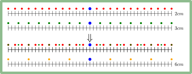
This was not special just to 2 and 3, and we can, for example, do it to the eight waves at lengths 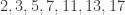$2,3,5,7,11,13,17$ and $19$ cm, so if we know what is $n$ modulo each of these length, then we know what it is modulo the multiplication. This multiplication is already pretty large

$2\cdot 3 \cdot 5\cdot 7 \cdot 11 \cdot 13 \cdot 17 \cdot 19 = 9,699,690\text{ cm} \sim 97\text{ km}.$

So with just 8 different types of waves, we satisfy out two conditions, and actually get the location modulo almost 100 km (unlike previously where we used $10^6$ types of waves to get only modulo 10 km).

The result that we just used is called the Chinese Remainder Theorem (CRT). In our notation above, we can formulate it as follows:

Definition: Two integers $a, b \in \mathbb{N}$ are called coprime if their greatest common divisor (gcd) is 1, namely if $d\mid a$ ( $d$ divides $a$ ) and $d \mid b$ , then $d=\pm 1$ .

The Chinese Remainder Theorem: Let $a,b$ be two coprime integers. Then for any $r_a,r_b \in \mathbb{N}$ there is some $r_{ab}\in \mathbb{N}$ such that if $n\equiv _a r_a$ and $n\equiv_b r_b$ , then $n \equiv_{ab} r_{ab}$ .

In particular, distinct prime numbers are always coprime, so in our radar example, if we know what is $n$ modulo these 8 different primes, then the CRT tells us that we know what is $n$ modulo their product.

Before we prove CRT, we need a lemma which characterize coprime numbers. This lemma is usually seen in the first abstract algebra course you take (and sometimes even sooner), and is part of a much bigger theory of algebraic structures. However, I will show here only an elementary proof, without going into the theory behind it. In general, some of the ideas below might seem weird to someone who never learned any abstract algebra, though all of them are quite natural when learned in a proper way (and I might even write a post about it some day…).

Lemma: Let $a,b\in \mathbb{N}$ . Then $a,b$ are coprime if and only if there are $m,k\in \mathbb{Z}$ such that $am+bk=1$ .

Proof: Assume first that we can find $m,n$ such that $am+bk=1$ . If $d\mid a,b$ , then it also divide the linear combination $d \mid am+bk =1$ , and the only integers which divide 1 are $\pm 1$ . In other words, we get that $a,b$ are coprime.

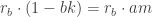
On the other hand, assume that $a,b$ are coprime, and let $d$ be the smallest positive number which we can write as $d=am+bk$ . If we can show that $d$ divides both $a$ and $b$ , then it must be 1 and we are done. We can always divide $a$ by $d$ and get a remainder, namely $a = qd+r$ where $0\leq r <d$ . This means that

$r = a-qd=a-q(am+bk)=a(1-qm)+b(-qk)$ .

We chose $d$ to be the smallest positive combination of $a,b$ , and since $0\leq r<d$ we conclude that $r=0$ , or in other words $d$ divides $a$ . The same argument works for $b$ , so that $d$ must divide both $a$ and $b$ and we are done. $\blacksquare$

Now that we have this lemma, we can prove the CRT.

Proof (Chinese Remainder Theorem): Assume that $a,b$ are coprime and find $m,k\in \mathbb{N}$ such that $am+bk=1$ . We first want to show that there is some integer $r$ such that $r \equiv_a r_a$ and $r \equiv _b r_b$ . The main trick is to note that $bk=1-am$ is divisible by $b$ on the one hand, namely it is zero modulo $b$ , but on the other hand it is 1 modulo $a$ . This means that $r_a \cdot bk =r_a \cdot (1-a_m)$ is zero mod $b$ and $r_a$ mod $a$ . We do the same trick with $r_b \cdot (1-bk) = r_b \cdot am$ and we get that

$r_{ab} = r_a \cdot bk + r_b \cdot am$

satisfy both of our conditions (You should check this and make sure that you understand what happened here).

Now that we have at least one solution, we want to find all the other solutions. Lets say that there is another solution $r$ to both of our conditions and write $\ell = r-r_{ab}$ . You can then check that $\ell=r-r_{ab}\equiv _a r_a -r_a =0$ and similarly $\ell\equiv_b 0$ , so that $\ell$ is divisible by both $a$ and $b$ . We claim that this means that $\ell$ is a multiple of $ab$ which by our notations means that $r\equiv _{ab} r_{ab}$ which is exactly what we wanted to prove.

By our assumption, we can write $\ell=\ell_1 a=\ell_2 b$ with $\ell_1,\ell_2 \in \mathbb{Z}$ . We can now get that

$\ell =\ell \cdot 1 =\ell \cdot (am+bk) = \ell_2 m \cdot ab +\ell_1 k \cdot ab = (\ell_1 k+ \ell_2 m)\cdot ab,$

so that $\ell$ is a multiple of $ab$ and we are done. $\blacksquare$

As I said before, the proofs above might seem like tricks to people unfamiliar with abstract algebra, though once one is used to the language and objects in this area, the process above becomes much more natural. In any way, we have only used some elementary congruence relations to prove the CRT, proving that our computation in the example of the radar was correct.

Even if you didn’t follow all of the computations above, there is one idea that is very important here. What the CRT tells us, is that if we want to solve the big problem of finding what is $n$ modulo $ab$ , then it is enough to solve the two smaller problems of modulo $a$ and modulo $b$ . In other words, this approach is a sort of divide and conquer approach. If the smaller problems are easier (as it is usually the case) and we have such a theorem that tells us how to combine them all together, then we can usually use this approach to solve the bigger problem.

Congruence problems are quite common in mathematics, so that this divide and conquer approach in the CRT make it very useful, in particular in problems in number theory. In particular, what we usually do it to “divide” our congruence problems to modulo prime power (for example mod $60$ to mod $2^2$ , mod $3$ and mod $latex 5%), and then hope that we can solve the problem for each prime power case.

The CRT also has a more generalized form which is applicable in other places. For example, a very common process in the general sciences is polynomial extrapolation. Namely, there is a polynomial of some fixed degree that we want to find, but we are not given all the information about this polynomial (i.e. all the coefficients). On the other hand, we are given some “local” information – the value of the polynomial at certain points. A very early result in the studies of probably every engineering student is that a polynomial of degree $d$ has at most $d$ roots. This quickly implies that if two polynomials of degree $\leq d$ have the same values at $d+1$ distinct points, then they must be the same. Once formulated in the language of rings, this results can be immediately seen to be a very close relative of the CRT we showed above, and actually the generalization of CRT almost includes this result.

One can even take this approach much further. Indeed, in the base of it, the Fourier transform which is used in signal processing all around the world, is just an infinite dimensional type of CRT. The Fourier transform tells us that when ever we have a periodic function (which is usually what we send in all those information wires which connect most of our thinking machines), this periodic function can be decomposed into “parts” which are the sines and cosines. Again, we see the usefulness of the divide and conquer approach – it is usually hard to work with a difficult periodic function, however it is much easier to work with a specific sine (or cosine) function.

In general, once you are used to working on mathematical problems (and problems in general), you learn to look for divide and conquer type results which decompose your problems to it basic blocks, in the hope that you can understand these blocks better. In particular, in the CRT we decompose to product coprime numbers. Since the product of small numbers can still be very large, what managed to show that with a very few different types of waves, we can get a lot of information.

2 Responses to Radars and the Chinese Remainder Theorem

Blais Black Smith says:

May 9, 2020 at 21:05

Reblogged this on FPGA Base X and commented:
Wonder whether this can be used to triangulate a WiFi or Bluetooth device by reproducing the originally sent data from the package and then comparing it to what has been received. Then doing the CRM for coprime wavelengths within the given package!

Blais Black Smith says:

May 9, 2020 at 21:08

Love this post. Had a similar idea for COVID-19 distance monitoring – in theory.