Linearity testing: Checking proofs for the lazy person

Taking a final exam in a course is not really a celebration cause for most students, but it is just not as fun to be on the other side as exam checkers. It can easily take several days to grade the answers for the same question for hundreds of students. The exam checkers would probably tell you that by just reading a few lines from the answer they know if it is going to be (mostly) correct or not, however they still need to read all of it just to be sure. These couple of lines can still be misleading – a good start can still lead to a complete failure, and a bad start might eventually, somehow, get most of the details right.

So maybe when checking exams we cannot really do it, but are there problems where reading only few lines from a proof is enough to determine its correctness? As it turns out, certain problems have innate structures that makes them more “stable” than others – if you write a “wrong” solution for them, then you can see it almost everywhere, so reading just a few lines will be enough.

One of the best examples for this kind of problem is the linearity testing. Suppose that someone claims that a function $f:\mathbb{F}_2^n \to \mathbb{F}_2$ is linear, and to prove it they show that $f(u)+f(v)=f(u+v)$ for all $u,v \in \mathbb{F}_2^n$ . What Blum-Luby-Rubinfeld (BLR) showed that in a sense it is enough to know that one of this conditions (chosen randomly) is true to conclude that all of them are true with high probability. In this post we will try to see what is so important about linearity, and which structures hides in this problem, to make this miracle happen.

Probabilistic proofs

As it is usually the case, our story starts with the famous linearity testers – Alice and Bob. Bob has a function $f:\mathbb{F}_2^n \to \mathbb{F}$ , which he claims to be linear, namely $f(u+v)=f(u)+f(v)$ for any two vectors $u,v\in \mathbb{F}_2^n$ . Alice, who needs some convincing, chooses two such vectors $u_0,v_0$ randomly, and checks that $f(u_0+v_0) = f(u_0)+f(v_0)$ . If true, she will accept the function as linear and otherwise reject it.

Of course, if $f(u_0+v_0) \neq f(u_0)+f(v_0)$ , then $f$ is not a linear function so Alice was right to reject it. However, $f$ might still be not linear, even if $f(u_0+v_0) = f(u_0)+f(v_0)$ , so Alice might be wrong claiming that it is. The question is what is the probability that she is wrong in this case.

Suppose Bob actually computed a linear function $f$ , but got a few mistakes along the way, so that the new function $\tilde{f}$ is not linear, but very “close” to being linear. In this case, the chances that Alice chooses one of these corrupted values is very small, so even though $\tilde{f}$ is not linear, with high probability Alice will say that it is. This is a problem that we can’t really overcome, and in general it doesn’t matter too much in practice. Alice will probably not use all of the values of the function, so there is a good chance that she will not even see the corrupted values. Further more, if $\tilde{f}$ is close enough to a linear function, Alice might be able to fix its problematic values.

The question becomes interesting when Bob doesn’t really start from a linear function, and his function $\tilde{f}$ is far from any linear function (for example, this can happen if Bob didn’t really study to the test, and just chose the function randomly). If this is the case, what is the probability that Alice is going to reject? For example, if for every linear function $f$ , Bob’s function $\tilde{f}$ has at least 5% of its values different than $f$ , then can we expect Alice to have more or less at least 5% chance of rejecting the function?

This miracle property is called the Soundness of the problem. Let’s give a more formal definition.

Definition: Given two functions $f,g:\mathbb{F}_2^n \to \mathbb{F}_2$ , we define their Hadamard distance by $dist(f,g) = {\displaystyle \frac{1}{2^n}|\{ v\in \mathbb{F}_2^n : f(v)\neq g(v)\}}$ . In other words, $dist(f,g)$ measure the chance of choosing a vector on which $f$ and $g$ disagree, and in particular $f=g$ if and only if $dist(f,g)=0$ .
For a set $W$ of functions, we write $dist(f,W)= \min_{g\in W} dist(f,g)$ .

With this definition, we want to show that following:

Theorem: Let $Linear$ the set of linear functions. Then for any $f\notin Linear$ , the probability $Prob_{u,v}(f(u+v)\neq f(u)+f(v))$ is at least $dist(f,Linear)$ .

In other words, if $f$ is far from being a linear function, then there is a good chance that Alice will notice. Note that Alice can always repeat this protocol to increase her chances to reject the function in case that it is not a linear function. Even if she is wrong with probability $0.95$ , she can run the protocol 100 times to lower her chance of being wrong to less than $0.01$ (and 100 checks is usually much less than the full $2^{2n}$ checks).

From simple to complicated

Many times, when facing a new problem, one of the biggest road blocks is where to start analyzing it. One of the approaches that I have found useful over the years, is trying to start with a more simplified version to get some intuition and after that add the structure back until returning to the original problem. This can be done, for example, by looking at a specific simple case of the problem, or, as I will do here, simplify the language that we use to study it.

Set Theory

In mathematics, one of the most simplest of languages is that of set theory. In this world of sets, and in particular of finite sets, the first question we should try to answer is what is the size of the sets. Our problem contains two sets – the set of all functions, and the linear functions

$\Omega = \{f:\mathbb{F}_2^n \to \mathbb{F}_2\}$ ,

$\Omega_0 = \{f \mid \;f(u+v)=f(u)+f(v) \; \; \forall u,v\}$ .

Let us start with studying $\Omega$ and then move to $\Omega_0$ .

In general, determining the size of sets is not an easy task. However, in our case the set $\Omega$ has a very unique structure. It is the set of all functions from $\mathbb{F}_2^n$ to $\mathbb{F}_2$ . This means that its size is $|\mathbb{F}_2|^{|\mathbb{F}_2^n|}$ , so if we know the sizes of both of these source and target sets, we can compute the size of $\Omega$ . Note that $\mathbb{F}_2^n$ in itself is also a set of functions (from $\{1,2,...,n\}$ to $\mathbb{F}_2$ ) so we can use the same trick here as well, and conclude that:

$|\mathbb{F}_2^n|=2^n \; \; \; ; \; \; \; |\mathbb{F}_2|=2 \; \; \; ; \; \; \; |\Omega|=2^{(2^n)}.$

Algebra

After set theory, the next language we should use is the one of linear algebra. While it can be very technical at times, it is quite easy to work with (and there is a reason that it is usually studied at the first semester). Our three sets from above, $\mathbb{F}_2^n, \mathbb{F}_2$ and $\Omega$ are actually vector spaces over $\mathbb{F}_2$ . When you start seeing vector spaces, you should always look for their dimensions as well, which in a sense, together with the field, determine the vector space completely. In particular, over the field with two elements, the dimension is just $\log_2(|V|)$ , so we get that:

$dim(\mathbb{F}_2^n)=n \; \; \; ; \; \; \; dim(\mathbb{F}_2)=1 \; \; \; ; \; \; \; dim(\Omega)=(2^n).$

Symmetry and Geometry

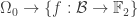
Next in our journey, we will look for all sorts of symmetries that our objects have. To get some intuition and be able to visualize the objects, lets restrict our problem to the $n=2$ case. In this world, our first set is just $\{(0,0), (0,1), (1,0), (1,1)\}$ which are just the vertices of the unit square. We can visualize the target set $\mathbb{F}_2=\{0,1\}$ as the black and white colors, so that a function $f\in \Omega$ is simply a colored square:

The importance of this visualization is that these sets have a lot of interesting natural symmetries like the rotations or reflections of the square, and these are closely connected to our objects.

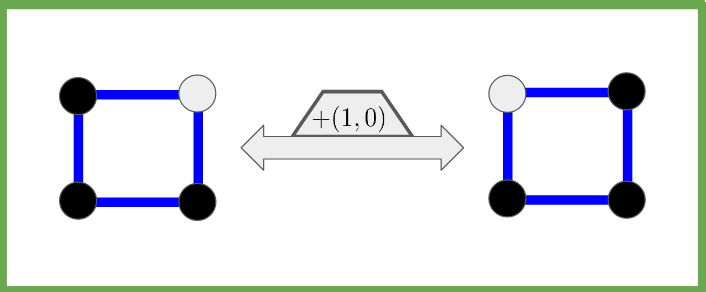
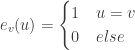
Since our sets are actually vector spaces, they come with the natural addition operations which act on them. For example, in our black\white visualization of the set $\mathbb{F}_2$ , adding $0$ does nothing, while adding $1$ flips between the colors. The addition in $\mathbb{F}_2^2$ in the geometric presentation, acts on the vertices. Here too adding $(0,0)$ does nothing, but for example adding $(1,0)$ switches between $(0,0) \leftrightarrow (1,0)$ and $(0,1) \leftrightarrow (1,1)$ , and in our square presentation this is simply the left to right reflection:

Similarly, adding $(0,1)$ is the up-down reflection, while adding $(1,1)$ is the rotation of 180 degrees.

Once we have these symmetries on $\mathbb{F}_2$ (switch colors) and on $\mathbb{F}_2^2$ (reflections and rotation), we can apply them to our colored squares in $\Omega$ to get, for example, this:

This is already a lot of interesting information, and we haven’t even started to look at the linear functions. The hope is that we can use each of these worlds of set theory, algebra and symmetry on these linear functions and combine it with what we saw on this larger set of all binary functions to produce some interesting results.

Describing the linear functions

Set theory of Linear functions

The set of linear function is defined by the linearity condition, namely

$\Omega_0 := \{f: \mathbb{F}_2^n\to \mathbb{F}_2 \mid \;f(u+v)=f(u)+f(v)\;\forall u,v\in\mathbb{F}_2^n\}$ .

Unlike the set of all functions, we cannot easily use this presentation to find the size of this set. However, this definition of linear function is not random, and it is rooted deeply within the algebraic structures of all of our sets. In particular, one of the first results that we learn on such functions, is that linear functions are determined completely by their values on a given basis of the vector space. Alternatively, every function from a basis can be extended uniquely to a linear function. Putting it more formally, if $\mathcal{B}\subseteq \mathcal{F}_2^n$ is a basis, then the restriction $f\to f\mid_\mathcal{B}$ to this basis, which is a map $\Omega_0 \to \{f:\mathcal{B}\to\mathbb{F}_2\}$ is a one to one and onto function. This new set is a “set of all functions”, so we can compute its size

$|\Omega_0| = |\mathbb{F}_2|^{|\mathcal{B}|} = |\mathbb{F}_2|^{dim(\mathcal{F}_2^n)}=2^n$ .

Algebra of Linear functions

The size of $\Omega_0\subseteq \Omega$ equals exactly to the dimension of $\Omega$ , which immediately raises the question whether it is a basis for $\Omega$ , which is nice to know in the land of algebra. However, we can quickly discard this idea since the set of linear functions is closed under addition, or in other words – it is a subspace (while in a sense a basis is a set “as far away as possible” from being close under addition). This might be disappointing a bit, but the property of being a subspace comes with its own advantages, and this coincidence of having the same size as a basis might (and will!) come handy in the future.

The symmetries of Linear functions

Returning to our $n=2$ case, we know that there are $4=2^2$ linear functions, and we can find and visualize them as colored squares (white=0, black=1):

What happens if we apply our reflections and rotation on these linear functions? No matter what we do to the full white square (the trivial function) it remains in place. However, if we apply them to the second colored square, the up-to-down reflection keeps it in place, but the left-to-right reflection and the 180 degrees rotation do not. But not all is lost – these two transformations are the same as simply switching the colors (which is the symmetry which comes from the addition in $\mathbb{F}_2$ !). The same happens with the other two linear functions. So in a sense, we should probably look at the pairs of functions:

In mathematics, when we have some action on a set, as above, and an element doesn’t change under this action (like the black\white square), we say that it is invariant under this action. The nontrivial linear functions are not invariant, but they are really close – they are invariant up to the color change. These “almost invariant” elements tend to appear in many places in mathematics, from simple examples like these rotating squares to the most advanced parts of mathematics.

If you are reading this post, then there is a good chance you already know some of these “almost invariant” objects really well. Indeed, maybe the best example for this behavior is when a linear transformation $T$ acts on a vector space $V$ . The simplest behavior we can hope for is to find $v\in V$ such that $T(v)=v$ , since then, for example, we can immediately compute $T^k(v)$ . However, since this is a very restrictive condition, we look for a more general definition where we only require that $T(v)=\lambda\cdot v$ for some constant $\lambda$ , or in other words – we look for eigenvectors. These “almost invariant” vectors are simple enough so that we could work with them, with a condition not too restrictive so they would actually exist, and as we shall soon see, this is exactly what we have in our problem.

The eigenvectos

In our problem, the posible eigenvalues are $\{0,1\}=\mathbb{F}_2$ , so eignevectors are either sent to $(0,0)$ , or are completely invariant, which is not good enough to describe our linear functions. The almost invariance up to the color switch means that $f$ is either sent to itself, or to the function $v\mapsto f(v)+1$ , so we add the scalar rather than multiply by it. Luckily for us, this is not too much of a problem, since we can use the standard trick to move from addition to multiplication – apply the exponent function.

Instead of working with $\mathbb{F}_2=\{0,1\}$ , we think of these two elements as $(-1)^0$ and $(-1)^1$ respectively, to get the set $\{+1,-1\} \subseteq \mathbb{R}$ . Converting our addition to multiplication, our sets become

$\Omega \to \tilde{\Omega} = \{f:\mathbb{F}_2^n \to \{\pm 1\} \}$

$\Omega_0 \to \tilde{\Omega}_0:=\{ f:\mathbb{F}_2^n \to \{\pm 1\} \mid f(u+v)=f(u)\cdot f(v) \; ;\; \forall u,v\}$ ,

both of which are contained in the $\mathbb{R}$ -vector space

$W:=\{f:\mathbb{F}_2^n \to \mathbb{R}\}$

of dimension $2^n$ . At least in the $n=2$ case, our arguments from above show that $\tilde{\Omega}_0$ are eigenvectors for all of our square symmetries (reflections and rotation). For the more general case:

Definition: For $v_0 \in \mathbb{F}_2^n$ , define the linear transformation $T_{v_0}:W\to W$ by $T_{v_0}(f) (u):= f(v_0+u)$ .

Claim: For any $v_0\in\mathbb{F}_2^n$ , and a multiplicative linear function $f\in\tilde{\Omega}_0$ we have that $T_{v_0}(f)=f(v_0) \cdot f$ – namely $f$ is an eigenvector with eigenvalue $f(v_0)$ .

Proof: Follows immediately from

$T_{v_0}(f)(u) = f(v_0+u) =f(v_0) \cdot f(u) \; \; \Rightarrow \; \; T_{v_0}(f) = f(v_0)\cdot f$ .

Now we are at a point where we have a set $\tilde{\Omega}_0$ consisting of only eigenvectos, and has exactly the size of a basis, which begs the question – is it a basis (over $\mathbb{R}$ ), and therefore make our symmetries diagonalizable?

Orthogonality

To prove that $\tilde{\Omega}_0$ is a basis, it is enough to show that it is an independent set. We can show it directly for any fixed $n$ by doing some manual computations, but this looks like too much work. Instead, lets try to extract some more information from our new visualization:

We already mentioned that these colored squares are almost invariant, but there is actually an even simpler property that we can see. The number of black and white vertices is always even, and while in the trivial function all the vertices are white, in the rest the number of black vertices equals to the number of white vertices. Now, after we moved to the $\pm 1 \in \mathbb{R}$ values instead of $\{0,1\} = \mathbb{F}_2$ , this is equivalent to having the sum of the values equal zero – exactly two $+1$ values and two $-1$ values.

What can we say about such vectors? For $n=2$ we are in a $4=2^2$ -dimensional space, which is a bit harder to visualize, so lets go even smaller to $n=1$ , in which case our two linear functions are the trivial function, which has values $(1,1)$ and the only non trivial linear function which has values $(1,-1)$ . In the plane they look like this:

The two vectors representing the functions have the same length, but more importantly they are orthogonal to each other. If we can show that in general the linear functions form an orthogonal set, then we automatically get that they are independent, and since it is a set of the size of the dimension of our vector space, they must form a basis.

As we shall see soon, “moving” from one linear function $\varphi$ to another $\psi$ equals their ratio $\frac{\psi}{\varphi}$ which is (multiplicative) linear in itself. Measuring the cosine of the angle is going to be the sum of the values, so unless $\varphi=\psi$ we expect to get 0, so that the functions must be orthogonal.

Orthogonality formalization

To prove this claim, we start with the definition of our inner product.

Definition: For two functions $f,g:\mathbb{F}_2^n \to \mathbb{R}$ we define their inner product as

$\left\langle f,g\right\rangle = \frac{1}{2^n} \sum_{v\in \mathbb{F}_2^n} f(v)g(v)$ .

With this definition in mind, lets see what we can say about functions from $\tilde{\Omega}$ which have values in $\pm 1$ and in particular about linear functions.

The first immediate result is that $\left\Vert f \right\Vert :=\sqrt{\left\langle f,f \right\rangle} = 1$ , so they are all on the unit sphere. Next, by definition $\left\langle f,g \right\rangle= \left\langle 1,f\cdot g \right\rangle$ . If both $f, g \in \tilde{\Omega}$ , then so is their product $f\cdot g$ and the same hold for multiplicative linear functions in $\tilde{\Omega}_0$ . In particular, this product is trivial $f\cdot g=1$ if and only if $f=g$ . You can either try to prove it directly, or note that this is exactly equivalent to $\Omega$ and $\Omega_0$ being vector spaces (close to addition and the field is $\mathbb{F}_2$ ).

The inner product $\left\langle 1, f \right\rangle$ is simply $\frac{1}{2^n}\sum_{v\in\mathbb{F}_2^n} f(v)$ – the summation over all the values of $f$ up to out normalization. If $f=1$ , then it is simply 1. However, if $f\neq 1$ is multiplicative linear, it has exactly two values $\pm 1$ , and each one appears exactly half of the times (this is a group homomorphism), so that $\left\langle 1, f \right\rangle = 0$ . Putting all of this together we get that:

Claim: Let $f,g:\mathbb{F}_2^n\to \{\pm 1\}$ be any two functions. Then

1. $\left\Vert f \right\Vert = 1$ , and
2. If both functions are multiplicative linear, then

$\left\langle f,g\right\rangle =\begin{cases} 1 & f=g\\0 & else\end{cases}$

Corollary: The set of multiplicative linear functions $\tilde{\Omega}_0$ forms an orthonormal set in the set of all functions $\mathbb{F}_2^n \to \mathbb{R}$ and therefore forms a basis.

Back to linearity testing

Now that we have all this new information about binary functions and linear functions we can return to the original problem of linear testing.

In the original problem, we wanted to show that if a binary function $f:\mathbb{F}_2^n\to\{\pm 1\}$ is far from a linear (multiplicative) function in the Hadamard distance, then with high probability when choosing $u,v \in \mathbb{F}_2^n$ we will get that $f(u+v)\neq f(u)\cdot f(v)$ , and then Alice will reject the function. Both the distance and the condition are essentially described using the standard basis. Defining

$e_{v}(u)=\begin{cases}1 & u=v\\0 & else \end{cases}$ ,

we think of $\{e_v \mid v\in \mathbb{F}_2^n\}$ as the standard basis and we can write $f = \sum a_v e_v$ (where $a_v \in \{\pm1\}$ .

Combination of the standard basis’ elements where 1=white, 0=green and -1=black.

Note that this basis is almost orthonormal – its elements are perpendicular to one another, and all have length $\frac{1}{2^{n/2}}$ . Now, the Hadamard distance basically ask how many of the coefficients are different in this presentation. Or more formally, if $g = \sum b_v e_v$ with $b_v \in \{\pm1 \}$ , then

${\left\Vert f-g \right\Vert}^2 = \sum_v {\left\Vert (a_v-b_v) e_v \right\Vert}^2 = \frac{1}{2^n} \cdot 4\cdot |\{v \mid\; f(v)\neq g(v)\}| = 4\cdot dist(f,g)$ .

Similarly in the linearity condition, is “defined” using this basis, since we look at the coefficient of $e_u, e_v$ and $e_{u+v}$ .

However, we just saw that there is another basis, which consists of linear functions, so we can write our function as a combination of these vectors:

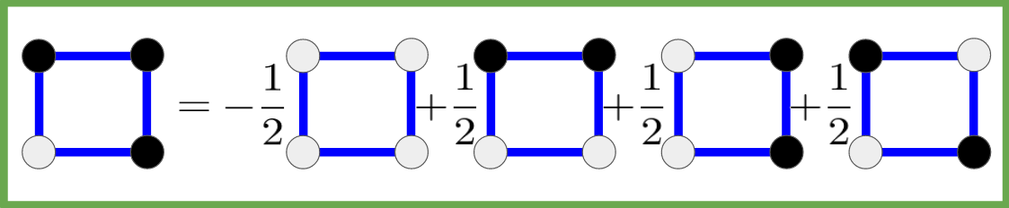
Lets denote these linear functions by $\{\varphi_1,...,\varphi_{2^n}\}$ , so we can write $f=\sum_i \alpha_i \varphi_i$ . If the function $f$ was a linear function, then the coefficients would all be zero, except one which will be $1$ . Using the orthonormality to our advantage, we also get that for any binary function

$1 = \left\langle f,f \right\rangle = \sum_i \alpha_i^2 \left\langle \varphi_i,\varphi_i \right\rangle = \sum_i \alpha_i^2$ .

It follows that if the function $f$ is not linear, then all of the coefficients would be in $[-1,1)$ . What can we say about the distance of the function from some linear function? While the distance was measured using the Hadamard distance, any orthogonal basis is just as good, so

$4\cdot dist(f,\varphi_i) = {\left\Vert f-\varphi_i \right\Vert}^2 = (\sum_{j\neq i} \alpha_j^2) + (\alpha_i-1)^2 = (\sum_j \alpha_j^2) -2\alpha_i + 1 = 2(1-\alpha_j)$ .

In other words, saying that the a function is far from all of the linear functions, is exactly saying that the $\alpha_i$ are far from $1$ , or more formally

$dist(f,Linear) = \frac{1}{2}\min_i (1-\alpha_i)$ .

We already see that in this new basis our distance function has a much simpler interpretation, and the main difficulty is to move from one base to the other, though this becomes simple if we can describe our expressions using inner products.

What about the probability for Alice to reject the function? If we can somehow rewrite it using the language of the inner product, we could move to this basis as well, and in this basis all the functions are linear, so it would be a much easier place to work in. And indeed we can rewrite it in the new basis and get that Alice will reject the function with probability at least $(1-\max_i \alpha_i)= dist(f,Linear)$ . For readability, I will put the proof in a new section, though it is very similar to what we saw here, but with extra details. The details themselves are less important than the idea of moving from a basis which is easier to describe the problem and the protocol to a basis which is easier to work with (and I encourage you to try prove it by yourselves).

The linearity condition

We would like to count how many pairs will lead Alice to reject the function. For a single $(u,v)$ pair, it is not hard to see that

$\frac{1-f(u)f(v)f(u+v)}{2}=\begin{cases}1 & f(u+v)\neq f(u)f(v)\\0 & else\end{cases}$ ,

so we want to sum over these expressions. Then the probability to reject will be

$Prob(reject)=\frac{1}{2^{2n}}\sum_{u,v} \frac{1-f(u)f(v)f(u+v)}{2} =\frac{1}{2}( 1 - \frac{1}{2^{2n}}\sum_{u,v} f(u)f(v)f(u+v)) .$

The term in the sum looks similar to an inner product, but has three factors instead of two, and have a double summation instead of a simple summation. As it turns out, this is because we have in a sense two inner products. First, we can define $F(u) = \frac{1}{2^n}\sum_v f(v)f(u+v)$ , so that

$\frac{1}{2^{2n}}\sum_{u,v} f(u)f(v)f(u+v) = \frac{1}{2^{n}}\sum_u f(u)\cdot F(u) = \left\langle f, F \right\rangle$ .

We would much prefer to work with the coefficients of $f$ in the basis of linear functions, since there we can see clearly the distance from linear functions. As for $F$ , since $+v=-v$ (it is in a vector space over $\mathbb{F}_2$ ), we can write it as $F(u) = \frac{1}{2^n}\sum_v f(v)f(u-v)$ which is an expression that appears many times in mathematics called a convolution and is denoted by $f*f$ . This convolution behaves like a function product in the sense that it is associative and distributive with respect to the function addition. But what is more important, is that the coefficient of $\varphi_i$ in the expansion of $f*g$ is the product of the coefficient of $\varphi_i$ in the expansion of $f$ times the coefficient in the expansion of $g$ (try to prove it!). Putting all of this together, we get that

$\left\langle f, F \right\rangle = \sum_i \alpha_i^3 \leq \max_i \alpha_i \sum_i \alpha_i ^2 = \max_i \alpha_i.$

This means that the probability for Alice to reject is

$Prob(reject) = \frac{1}{2}(1 - \frac{1}{2^{2n}}\sum_{u,v} f(u)f(v)f(u+v) )\geq \frac{1}{2}(1-\max_i\alpha_i)=dist(f,Linear) ,$

which is exactly what we wanted to show.

In conclusion: So what did we do?

Trying to analyze our problem, we looked for simple ways to describe its objects. We started with considering them as sets, then added the addition to get algebraic objects, and then used these addition operations to find symmetries and actions on our sets. When applying the same process to the linear functions, we concluded that they are also orthonormal eigenvectors which led us to a new interesting basis.

Then the main trick was moving from one basis to the other. The standard basis is what we usually work with, and it is easy to describe the problem in this basis (for example, the distance is measured by simply counting the number of different coefficients). However, the second basis is far more related to the essence of the problem – it is exactly the set of linear functions. Both bases were orthonormal (up to a uniform normalization), so when the expressions were transformed to use inner products, it was very easy to move from one to the other. Once we moved all of our notation to this new basis, the problem became almost trivial.

Along the way we also encountered the convolution operation, which behaved nicely with respect to this base change. You might have seen this sort of behavior in another place – the Fourier transform. This is not surprising, since this base change is the Fourier transform, and this interesting result about the convolution is one of the main reasons that the Fourier transform is so important.

All of these different structures, the bases, and the conversion between them were miraculously combined together to show that if Bob didn’t really make an effort to create a linear function, then Alice would have a good chance to detect it. It does, however, rely on the fact that Bob is honest. If Alice asked Bob for the values of $f$ on $u, v$ and $u+v$ , Bob could reply any three values of the form $a,b$ and $a+b$ (instead of $f(u), f(v)$ and $f(u+v)$ ) so that Alice will always accept. For this post, we would assume Bob’s honesty, but if we really wanted, we could change the protocol and have Bob commit to the answers before Alice asks for these values, but we will leave it for another post.

As a final thought, I would like to point out that this miracle combination happens a lot. After all, it is the basis for the Fourier transform that every engineer knows by heart, or its mathematical name – group representation. This in itself is a subject on its own, but once you understand its basics, results like those in this post become much more natural.