On one weird rational average

One of the things that I love about Mathematics, is how one can come across a mathematical problem or a phenomenon which you can look at from several points of views, each one different, yet they all combine together to form an interesting story. It can be a story that grows with you as you learn more and more advanced mathematics, or a story that lets you connect different parts of mathematics.

The story, which is the focus of this post and the next one, is a story of such a problem around the operation which takes two positive rational numbers $\frac{a}{b}<\frac{c}{d}$ and “returns” the wrong way to add them: $\;\;\frac{a+c}{b+d}$ . This story starts from the most elementary mathematics there is, and goes all the way to the most advanced, and on the way it introduces many interesting concepts in mathematics.

For all of you Hebrew speakers out there, a video version of this posts can be found here: https://www.youtube.com/watch?v=SPFxgNcm5rs

A new interesting average.

I first learned about this operation when I was in elementary school. At the attempt of trying to teach us the pupils mathematics, the school had a very simple math computer game for us to play. In this game there was a man walking in a hallway and each time he wanted to open a door, he needed to find a rational number between two other rationals.

For example, we can get the problem of finding a rational number $q$ such that

$\frac{1}{5} < q < \frac{2}{3}.$

There are many ways to find such a rational number, but probably the most well known is to go for the number exactly in the middle, or in other words the arithmetic mean:

$q = \frac{\frac{1}{5}+\frac{2}{3}}{2}=\frac{1\cdot 3 +2\cdot 5}{2\cdot 3\cdot 5}=\frac{13}{30} .$

Once one door is opened, the next two rationals will be $q$ and one of the previous rationals, for example, find:

$\frac{13}{30} < ? < \frac{2}{3}.$

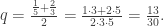
Repeatedly computing these arithmetic means will not only teach the pupils about their importance, but also teaches them how to add rationals (e.g. computing $\frac{1}{5}+\frac{2}{3}$ ), and along the way compute 4 multiplications and 1 addition of integers. As learning tools go, this can be a very good one to learn addition and multiplication.

As a future mathematician, and a lazy person, I somehow found out that if I just add the numerators and denominators, I get a rational somewhere in the middle, for example:

$\frac{1}{5} < \overbrace{\frac{1+2}{5+3}}^{3/8} < \frac{2}{3}$

This meant that not only I had to compute only 2 additions, but also, as can be seen in the examples above, both the numerator and the denominator 3 and 8 are much smaller than their counterparts 13 and 30 in the arithmetic mean. This means that the next step will be even easier since I need to deal with smaller numbers.

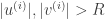
Formally speaking, years after finishing elementary school and a couple of degrees in mathematics, the claim above is that given two rationals $0\leq\frac{a}{b}<\frac{c}{d}$ we have that

$\frac{a}{b}<\frac{a+c}{b+d}<\frac{c}{d}$ , and
The numerator and denominator of $\frac{a+c}{b+d}$ are “small”.

While the second claim is more intuition than an actual formal claim, the first one can be easily checked to be true. This is a very simple exercise – since all the denominators are positive, we have that

$\frac{a}{b}<\frac{a+c}{b+d} \iff a(b+d)<b(a+c) \iff ad<bc \iff \frac{a}{b}<\frac{c}{d}$ ,

proving the left inequality in (1) above, and a similar argument proves the right inequality. In other words, the weird sum $\frac{a+c}{b+d}$ is a some kind of an average of $\frac{a}{b}$ and $\frac{c}{d}$ . But easy as the proof may be, it doesn’t give us any intuition about why it is true, why should we care about this average and why it is interesting.

Being in elementary school, I didn’t even know that I needed to ask these questions, and I mostly forgot about this operation up until my post doc.

A rational postdoc conversation

In my postdoc, one of the problems that came up in my research was about distribution of rationals in all sorts of places. For example, the most “standard” way in which we think about rationals distribute inside the real line $\mathbb{R}$ is to fix the denominator $n$ and then look on all the rationals with that denominator $\Omega_n=\{\frac{k}{n} \mid k\in \mathbb{Z}\}$ . For example, on the unit segment we have the following:

After managing to prove some interesting claims for the distribution of rationals above, in my postdoc I was asked if I could do it for other distributions as well. Of course, this is very much dependent on which distribution. Then, it was suggested that I try to use a special way of ordering the rationals, which for my surprise meant that I will need to use this weird operation that I used in elementary school.

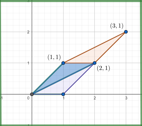
The method was as follows. Start with the rationals zero and one, but write them as $\frac{0}{1}$ and $\frac{1}{1}$ . Then add the numerators and denominators to get the three rationals: $\frac{0}{1}, \frac{1}{2}, \frac{1}{1}$ . Next step create new rationals by adding numerators and denominators of each consecutive pairs to get $\frac{0}{1}, \frac{1}{3}, \frac{1}{2}, \frac{2}{3}, \frac{1}{1},$ and we can continue this step again and again infinitely many times.

Once I heard about it in the postdoc, I learned that this weird summation is called the mediant. In the picture above, we wrote each mediant $\frac{a+c}{b+d}$ between its “summands” $\frac{a}{b}$ and $\frac{c}{d}$ . Since we already showed that $\frac{a}{b}<\frac{a+c}{b+d}<\frac{c}{d}$ , then the numbers above are also ordered by their size, and in particular all the numbers that we can create like this are different. This in itself is already interesting, even though easy to prove, but then I was told that this process is much more interesting:

Theorem: Every rational number in $[0,1]$ appears in this repeated mediant process.

This is already a much more powerful theorem than just proving that the mediant computes some average of two rational numbers.

Forgetting for a moment my elementary school days, I have basically never heard about these mediants, let alone this theorem. However, the moment I saw it, I knew that I can prove it. More than that – it felt like I knew everything about this operation and the theorem, except that it existed.

But this is not enough – the 10 year old in me could not understand the university level mathematics, so I needed to find a way to prove it in the most elementary way that I can find, and this is exactly what I am going to do in this post, and in the later posts I will show how this same problem leads to more and more mathematics.

Start from the definition

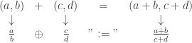
One of the first thing that you learn to ask in mathematics is if a new definition is “well defined”. For example, in the standard rational addition we have 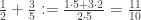$\frac{1}{2} + \frac{3}{5} := \frac{1\cdot 5 + 3\cdot 2}{2\cdot 5} = \frac{11}{10}$ . The rational $\frac{1}{2}$ has many presentations, e.g. $\frac{1}{2} = \frac{2}{4} = \frac{3}{6} = ...$ , and at first look you might wonder if $\frac{2}{4} + \frac{3}{5} := \frac{2\cdot 5 + 3\cdot 4}{4\cdot 5}$ also equals to $\frac{11}{10}$ . In other words, is the addition operation depends on the rational numbers themselves, or their presentation. If it is not defined by the value of the numbers, but by their presentations, then by definition it is not well defined.

While the standard rational addition is well defined – changing the presentation doesn’t change the result – the mediant is not well defined. If we write

$\frac{a}{b} \oplus \frac{c}{d} := \frac{a+c}{b+d}$ ,

then for example we have that $\frac{1}{2} = \frac{2}{4}$ and $\frac{2}{3} = \frac{6}{9}$ ,but

$\frac{1}{2}\oplus \frac{2}{3} = \frac {1+2}{2+3} = \frac{3}{5} \text{ while } \frac{2}{4} \oplus \frac{6}{9} = \frac{2+6}{4+9} = \frac{8}{13} \neq \frac{3}{5}.$

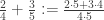
Already we reached our first roadblock – our operation is not well defined. However, we already know that it does have a special property – it computes some sort of average – so we need to somehow make it well defined, and then study it. Making an operation into a well defined one is usually quite simple. Instead of considering the objects themselves, consider their presentations as objects. In our case, instead of the rational number $\frac{a}{b}$ we think of the integer vector $(a,b)$ , and the rational number is the “projection” of this vector: $(a,b) \mapsto \frac{a}{b}$ .

Now, our operation in the world of integer vectors is simply the vector addition:

$\begin{array}{ccccc}\left(a,b\right) & + & \left(c,d\right) & = & \left(a+b,c+d\right)\\ \downarrow & & \downarrow & & \downarrow\\ \frac{a}{b} & \oplus & \frac{c}{d} & ":=" & \frac{a+b}{c+d} \end{array}$

and taking the projection of both side gives us the original (not well defined) “operation”. So while in the 1-dimensional rational context the mediant is not well defined, we see that it is actually a shadow of a well defined 2-dimensional integer operation. In general, 2-dimensional objects might be harder to deal with than 1-dimensional objects, but in this case we also moved from rationals to integers, but even better – we have a nice visualization for this whole process.

The geometric point of view

First, for the projection itself, the integer vectors mapped to the rational $q=\frac{a}{b}$ , are exactly the integer vectors on the line $L=\mathbb{R}\cdot (a,b):=\{(ta,tb):\; t\in \mathbb{R}\}$ . Moreover, if we intersect this line with the horizontal line $y=1$ , then the intersection point is exactly $(\frac{a}{b},1)$ . So in a sense, the rational $q$ is the “shadow” that the line $L$ drops on the line $y=1$ .

Now that we have the projection, we can also look at the addition:

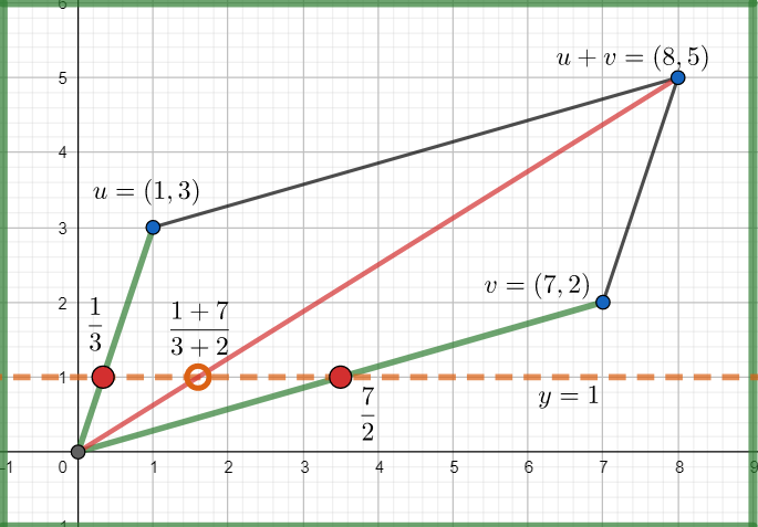
With the images above in mind, showing that $\frac{a}{b} < \frac{a+c}{b+d} < \frac{c}{d}$ is straight forward. We start with the segments from the points $(a,b), (c,d)$ to the origin (the green segments), and complete them to a parallelogram. The diagonal of this parallelogram (in red) is always inside it, and in particular between the two green lines, so when we project it onto $y=1$ , its projection $\frac{a+c}{b+d}$ is between the projections of these lines. In other words, we get the inequality from above.

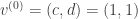
We already managed to convert one elementary computation to a visual, and intuitive, proof. Next, we want an even better result, and we shall use this visualization to show that we can get any rational number in $[0,1]$ when starting at $0,1$ and use the repeated mediant process.

To get some intuition, lets start with a simple process of getting from $\frac{0}{1}, \frac{1}{1}$ to $\frac{3}{5}$ . We first start by computing the mediant $\frac{0}{1} \oplus \frac{1}{1} = \frac{1}{2}$ to get the triple $\frac{0}{1} , \frac{1}{2} , \frac{1}{1}$ . We are looking for $\frac{3}{5}$ , and we need to decide if we look inside $(\frac{0}{1} , \frac{1}{2})$ or $(\frac{1}{2}, \frac{1}{1})$ . For our simple example we can just check which segment contains this point, but we are looking for intuition for the general case, so let view our geometric interpreation:

First step (with x,y coordinates switched for horizontal viewing)

As can be seen in the image above, the triple $\frac{0}{1} , \frac{1}{2} , \frac{1}{1}$ defines a parallelogram for us, and since we can see the line corresponding to $\frac{3}{5}$ , we know that we need to go down to the pair $(\frac{1}{2}, \frac{1}{1})$ .

Repeating this process we get the triple $\frac{1}{2} , \frac{2}{3} , \frac{1}{1}$ , go down to $(\frac{1}{2} , \frac{2}{3})$ and finish with the mediant of these two rationals which is $\frac{3}{5}$ . Visually we moved through these parallelograms:

Here we saw that we can get to $\frac{3}{5}$ , and in general we can try to use this process for any rational $0<\frac{n}{m} <1$ . The question is if this process always ends, or if there are cases where it does not. Intuitively, we expect the edges of the parallelograms to become larger and larger, and since the rational\integer point is always between the lines they define, if the process never stops, then eventually we expect to see this point inside the parallelogram. However, as can be seen in the images above, the parallelograms never contain integer points, and this will lead to a contradiction.

Before we give a formal proof for this result, let us define the repeated mediant process properly.

The mediant process

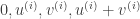
We start with two vectors $u^{(0)} = (a,b)=(0,1)$ and $v^{(0)} = (c,d)=(1,1)$ (corresponding to the rationals $0$ and $1$ ), and we want to reach some vector $w=(n,m)$ in between them (namely $\frac{0}{1}<\frac{n}{m}<\frac{1}{1}$ ). We also assume that $n, m$ are coprime (we can always consider our rational in its reduced form).

At each step, if $u^{(i)} + v^{(i)} = w$ , then we are done. Otherwise we look at the three vectors $u^{(i)} , u^{(i)} +v^{(i)} , v^ {(i)}$ . If the line defined by $w$ is between the lines corresponding to $u^{(i)} , u^{(i)} +v ^{(i)}$ , then in the next step we have $u ^{(i+1)} = u ^{(i)}$ and $v ^{(i+1)} =u ^{(i)} +v ^{(i)}$ . Otherwise, namely $w$ is between $u ^{(i)} +v ^{(i)}$ and $v ^{(i)}$ (linewise) and we continue to $u ^{(i+1)} = u ^{(i)} +v ^{(i)}$ and $v ^{(i+1)} =v ^{(i)}$ .

The process ends if we at some point reach $w$ and otherwise it is infinite.

In the language of the process above, the parallelograms that we see are those with vertices at $0,\; u^{(i)} ,\; v^{(i)},\; u^{(i)}+v^{(i)}$ . There is something very special when we move from the i’th parallelogram to the next. We can actually think of it as cutting the current parallelogram to two triangles, and then moving only one triangle by translating it in an integer direction.

We cut the (blue + purple) parallelogram, and move the purple triangle at direction (1,1) to become the orange triangle, and then glue it back together with the blue triangle.

The first immediate result from this point of view, is that all of our parallelograms have the same area, no matter how many steps we take. Indeed, when we cut a parallelogram to two triangles and then glue them together, we do not change the total area. The second result is that all of our parallelograms don’t contain integer points in their interior (only their vertices are integer points). More generally, if $S\subseteq \mathbb{R}^2$ is any set, and we look at its translate $(a,b)+S := \{ (a,b)+s : s\in S\}$ for some integers $a,b$ , then $S$ contains the integer point $(n,m)$ if and only if $(a,b)+S$ contains the integer point $(a+n, b+m)$ . It follows that $|S\cap \mathbb{Z}^2| = | ( (a,b)+S )\cap \mathbb{Z}^2|$ . In the case of our parallelograms, our initial parallelogram doesn’t contain any integer points, so all of the rest of the parallelograms don’t contain integer points as well.

We now have all the ingredients to show that we can reach any rational number by taking mediant steps.

Theorem: For any $w=(n,m)\in\mathbb{Z}^2$ such that $0<\frac{n}{m}<1$ , the mediant mediant process defined above eventually stops.

Remark: I tried to keep the following proof as elementary as possible. There are simpler, more elegant proofs using a bit of linear algebra which I will show in the next post. For now you are welcome to try and find such a proof.

Proof: Consider the parallelograms $P_i$ defined by $0, u^{(i)}, v^{(i)} , u^{(i)} +v^{(i)}$ . We expect these vectors to grow as $i$ increase. In particular, you should prove the if $|u^{(i)}| , |v^{(i)}| > R$ , then the section of the circle of radius $R$ between the lines defined by the vectors $u^{(i)} , v^{(i)}$ is completely inside the parallelogram. So if the process never stops, and these vectors increase enough in size, then eventually we could take $R=|w|$ , so that the integer point $w$ will be contained inside the parallelogram, which is a contradiction (hence, the process must stop at some point).

The blue area part of the circle is contained entirely in the parallelogram.

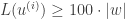
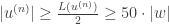
A simple way to track the size (more or less) of these vectors is by using the simple map $L((a,b)):=a+b$ . For $a,b\geq 0$ this map satisfies:

$|(a,b)|:=\sqrt{a^2+b^2}\geq \max\{a,b\}\geq \frac{a+b}{2} = \frac{L((a,b))}{2}$ .

Our initial vectors $u^{(0)}=(0,1)$ and $v^{(0)}=(1,1)$ have nonnegative entries. Since in our process we only add vectors, we always remain with nonnegative vectors so that the inequality above holds.

Additionally, we have the nice property that $L(u+v)=L(u)+L(v)$ , so if $L(u), L(v)\geq 1$ , then $L(u+v)\geq \max(L(u), L(v)) +1$ . Applying this result to our process, it is easy to check that $L(u^{(i)}+v^{(i)})\geq i+1$ for each $i$ . Finally, since at each step either $u^{(i)} = u^{(i-1)}+v^{(i-1)}$ or $v^{(i)} = u^{(i-1)}+v^{(i-1)}$ , then at least one of them has sum of coordinates equals to $L(u^{(i-1)}+v^{(i-1)})\geq i$ .

Suppose that we updated both $u^{(i)}$ and $v^{(j)}$ at some $i,j > 100\cdot |w|$ . At the point of update we know that $L(u^{(i)}) \geq 100\cdot |w|$ , and since $L(u^{(n)})$ is an increasing sequence, this inequality is true for all $n$ large enough. It follows that

$|u^{(n)}| \geq \frac{L( u^{(n)} )}{2} \geq 50\cdot |w|$

for all $n$ large enough, and the same holds for $v^{(n)}$ . But as we wrote in the beginning of the proof, this will lead to a contradiction where we have an integer point $w$ inside our parallelogram. We conclude that at least one of them is not updated at all after a certain point.

Without loss of generality, assume that $u^{(i_0)} = (a,b)$ , $v^{(i_0)} = (c,d)$ at some index $i_0$ and from this point on we don’t update $v$ . This means that $u^{(i_0 + k)} = (a,b)+k\cdot (c,d)$ and $v^{(i_0 + k)} = (c,d)$ for all $k\geq 0$ . Letting $w = (n,m)$ , by the definition of our process, we must have

$\frac{a+kc}{b+kd} < \frac{n}{m} < \frac{c}{d}\; , \; \forall k\geq 0$ .

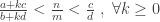
However, we can write $\frac{a+kc}{b+kd} = \frac{a/k+c}{b/k+d}$ which is almost $\frac{c}{d}$ (which is larger than $\frac{n}{m}$ ) when $k$ goes to inifnity, and we get our desired contradiction. Visually, what happens is :

We see that even if the $v^{(i)}$ are not updated after some point, we can’t continue the process for ever. In other words, the process must stop at some point, which is exactly what we wanted to prove. $\square$

Conclusion for my 10 years old past self

While the last proof became a little technical, the geometry behind it was quite simple. Hopefully it is simple enough so that my past self could understand most of it. However, this is only the beginning of the story. If you know a little bit of linear algebra, there is a good chance that you caught some glimpses of it along the way. In the next post, I will meet my past self from my Bachelor degree in mathematics and see how this same problem and results are connected to all sorts of mathematical subjects and connects them nicely together.